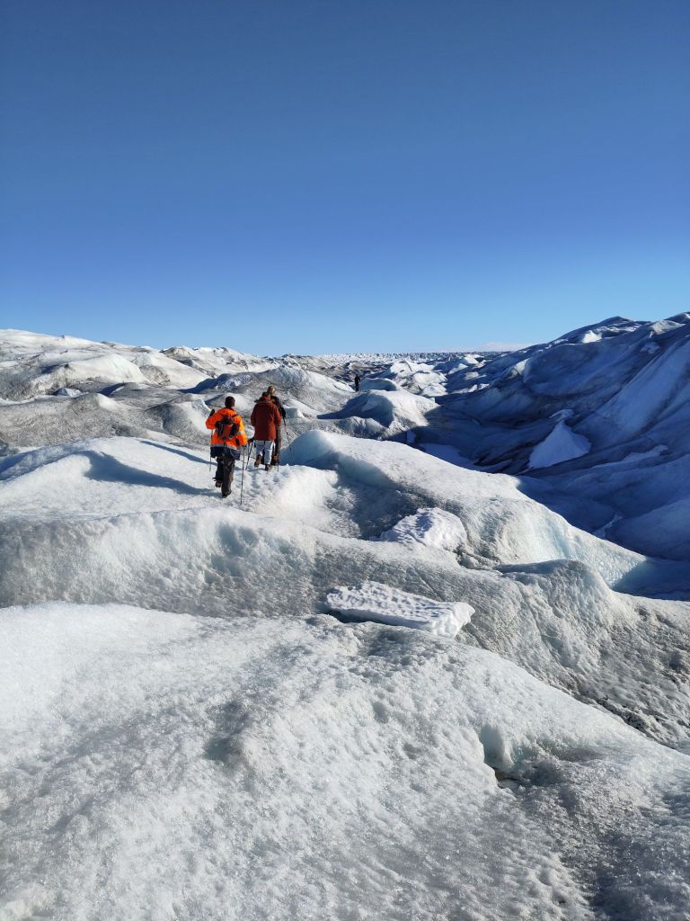
I’m a co-author on a new paper that has just come out in GRL. It’s based on simulations we did with our collaborators in the PROTECT project on sea level contributions from the cryosphere. What Glaude et al shows is that, to quote the first of the 3 key points:
“With identical forcing, Greenland Ice Sheet surface mass balance from 3 regional climate models shows a two-fold difference by 2100”
In perhaps more familiar terms, if you run 3 regional climate models (that is a climate model run only over a small part of the world, in this case Greenland) with identical data feeding in from the same global climate model around the edges, you will get 3 quite different futures. Below you can see how the 3 different models think the ice sheet will look on average between 2080 and 2100. The model on the right, HIRHAM5 is our old and now retired RCM. It has a much smaller accumulation area left by the end of the century than the other two, which have much more intense melt going on in the margins.

In fact, by the end of the century, although the maps above seem to show HIRHAM having much more melt, there is in fact more runoff from the MAR model, because of this intense melt.

The surface mass balance (SMB) at the present day is in fact positive. This often surprises people, but SMB as the name suggests, only describes surface processes. Ice sheets can (and do) also lose a lot of ice by calving and subglacial and submarine melt. As SMB should balance everything if a glacier is to remain stable or even grow, present day SMB is usually 300 to 400 GT positive at the end of each year, and even so the Greenland ice sheet loses, net around 270Gt per year.
Our work here shows that, at least under this pathway, not only does SMB become net negative in itself by the middle of this century, there are significant differences in SMB projections between the estimates of how negative it will be, between the three RCMs. The global model we used, CESM2 under the high-end SSP5-8.5 scenario, is famously a warm scenario, but our estimated end of the century SMBs are extraordinary : (−964, −1735, and −1698 Gt per year, respectively, for 2080–2099). As I’ve discussed previously, one gigatonne is a cubic kilometre of water, 360Gt is roughly 1mm global mean sea level rise. (Though note your local sea level rise is *definitely* not the same as global average!) Even the lowest estimate here the is giving around 3 mm of global average sea level rise from surface melt and runoff *alone* by the end of this century each year. That’s pretty close to the modern day observed sea level rise from all sources.
And this is in spite of the fact that at the present day, the 3 models are rather similar in their estimates of SMB. The Devil is as usual in the details.
We attribute these startling divergences in the end of the century results to small differences in 1) the way melt water is generated, due to the albedo scheme (that is how the ice sheet surface reflects incoming energy); 2) but also due to the cloud parameters that control long-wave radiation at the surface, which again can promote or suppress melting. (We really need to know how much liquid water or ice there are in clouds, as this paper also emphasises in Antarctica); and 3) mainly down to the way liquid water that percolates down from the surface is handled in the snow pack. That is, how much air there is in the snowpack, how warm the snow is and how much refreezing can occur to buffer that melt.
The problem is that all of these processes happen at very small scales, from the mm (snow grains and air content), to the micron scale (cloud microphysics). That means that even in high (~5km) resolution regional models, we need to use parameterisations (approximations that generalise small scale processes over larger spatial and/or time scales). Small differences between these parameterisations add up over many decades. Essentially, much like the famous butterfly flapping its wings in Panama and causing a hurricane in Florida, the way mixed phase clouds produce a mix of water vapour and ice over an ice surface might ultimately determine how fast Miami will sink beneath the waves.
More data would certainly help to refine these parameterisations. The main scheme to work out how much liquid can percolate into snow was originally based on work by the US Army engineers in the 1970s. More field data with different types of snow would surely help refine these. Satellite data will be massively helpful, if we can smoothe out some wrinkles in how clouds (there they are again) affect surface reflectivity.
These 3 different types of processes also interact with each other in quite complex ways and ultimately affect how much runoff is generated as well as the size of the runoff zone in each model. So integration of many different types of observations is crucial.
“Different runoff projections stem from substantial discrepancies in projected ablation zone expansion, and reciprocally” as we put it in Glaude et al., 2024.
The timing and magnitude of the expansion of the runoff zone is quite different between the models, but all of them show a very consistent increase in melt and runoff over the next 80 years.
It’s probably also important to understand a couple of key points:
Firstly we ran a very high emissions pathway: SSP5-85 is probably not representative of the path we will follow in emissions (at least I hope not), but in this study we wanted to address the spread on different model estimates. And this is a way to get a good check on the sensitivity.
Secondly, the ice sheet mask and topography in these runs is kept fixed all the way through the century. This means we do not account for any elevation feedbacks (as the ice sheet gets lower because of melt, a larger area becomes vulnerable to melt because it’s lower and thus warmer), but we also don’t account for ice that has basically melted away no longer contributing to calculated runoff later in the century. Ice sheet dynamics are also not factored in.
Finally, we ran different resolution models, and that can have an impact particularly on precipitation and is one of the reasons why the new models we developed and have run in PolarRES (and which are now being analysed), have used a much more consistent set-up.
The 3 models we used, MAR, RACMO and HIRHAM have all been used in many different studies over both Greenland and Antarctica, but we haven’t really done a systematic comparison of future projections before. I think this work shows we need to get better at doing this to capture the uncertainty in the spread, especially when you consider that we’re now looking at using these models as training datasets for AI applications: training on each one of these models would give quite different results long-term. We need to think about how to both improve numerical models and capture that spread better. But ultimately, it’s how fast we can reduce greenhouse gas emissions and bend the carbon dioxide curve down that will determine how much of Greenland we will lose, and how quickly.
All data and model output from these simulations is available to download on our servers (we’re transitioning to a new one download.dmi.dk, not everything has been moved there yet). We also of course have data over land points and the surrounding seas, and we’ve run many more global climate models through the regional system to get high resolution (5km!) climate data also looking at different emissions pathways, if you’re interested in looking at, analysing or using any of this data – get in touch!
My warmest thanks to Quentin Glaude who led this analysis and special thanks to our colleagues in the Netherlands, France and Belgium for running these models and contributing to the paper analysis. Clearly, we have much work to do to get better at this ahead of CMIP7.