Divergence


A new paper came out today, and in some ways it is the end of an era. But the results are also quite important both scientifically and for society.

Benjamin Heurgue and Charles Amory, both at the Institut des Géosciences de l’Environnement in Grenoble, have done a magnificent job, leading a comparison of future Antarctic surface mass balance from three different regional climate models, including our own HIRHAM5.

Our DMI contribution was actually rather small: we basically contributed simulations and a bit of analysis, while all the hard thinking was done in Grenoble (and of course by our good friends and colleagues in Brussels, Utrecht, Bergen, Liège and Oslo, I very much enjoy working in these international teams).
The concept of the paper is beautifully simple. Take one global climate model (CESM2) running one high-emissions scenario, and downscale it with three regional climate models — MAR, RACMO and HIRHAM5.

Regional climate models are like a magnifying glass over the ice sheet: they get the same large-scale weather from the global model, but each has its own way of handling what happens at the surface — snowfall, melt, refreezing and runoff.  The question Benjamin asked is: if we all start from the same place, do we end up in the same place?


For the present day: yes, reassuringly. All three models agree on today’s Antarctic surface mass balance — roughly how much snow falls, how much melts, and how much of that meltwater actually escapes. But by 2100 they diverge strongly, especially over the ice shelves. HIRHAM projects a large decline, MAR a moderate one, and RACMO stays close to balance. This might sound familiar. A similar paper led by Quentin Glaude about Greenland had a similar conclusion and as in that paper, the culprit is runoff.
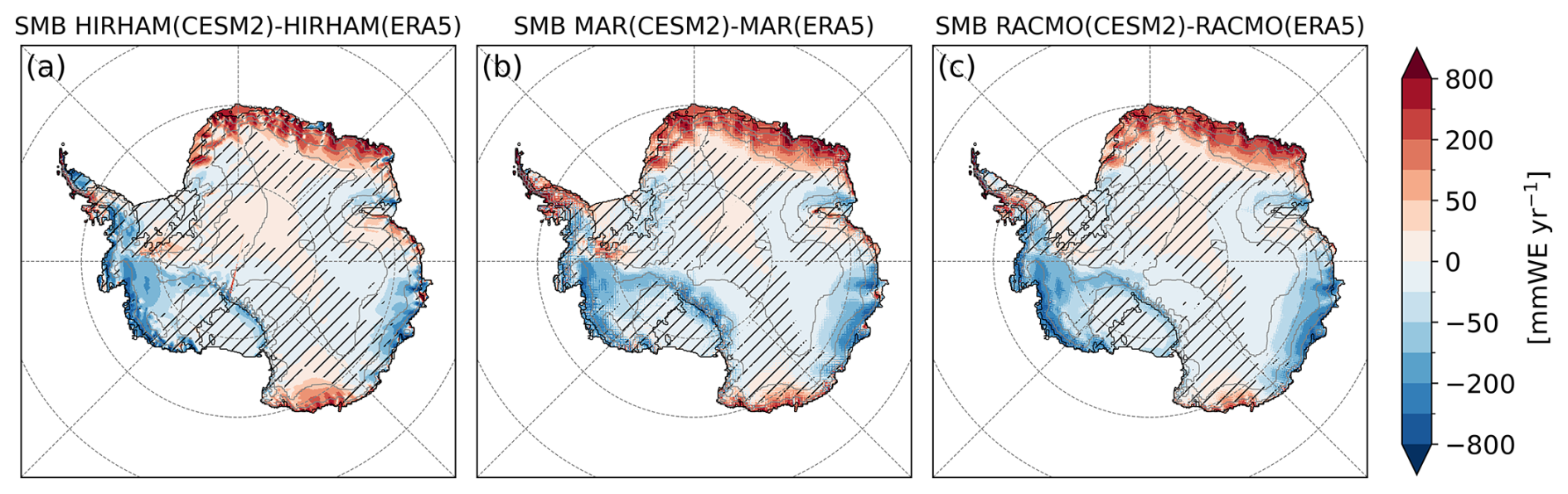
Figure 1 from the paper: Differences in mean Antarctic SMB simulated by the RCMs: HIRHAM (a), MAR (b), and RACMO (c), driven by CESM2 and ERA5, in , over the reference period 1995–2014. Hatched areas indicate regions where the differences are smaller than the interannual variability (standard deviation over the period) of the SMB from RCMs driven by ERA5. As you can see, there are some differences, but they are relatively small at present day.

If the three models broadly agree (very broadly) on the SMB components at the present day, there are also some.commonalities in the future projections. Over the grounded ice sheet all of them project more snow as the world warms, because a warmer atmosphere carries more moisture, but it’s both the amount of melt and the amount of runoff that they disagree on.
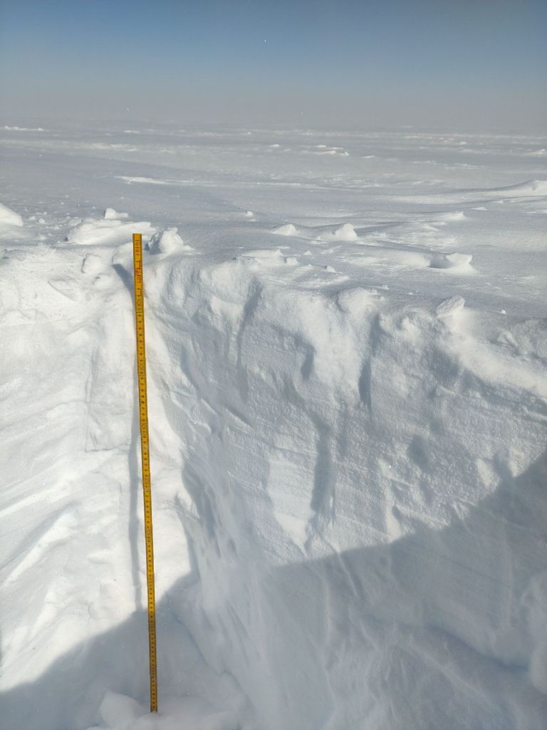
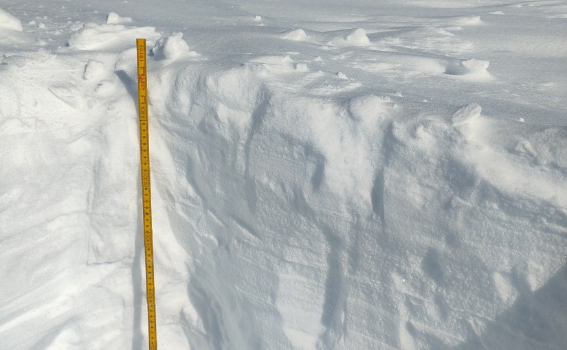
Snowpit on an ice shelf – the retention capacity of the snowpack and the firn is determined by temperature, density and other factors that we can measure in the field. This is one I dug on the Riiser-Larsen ice shelf last year.


The divergence is mostly about the snowpack or rather what we call the firn (the top several metres of old snow, all of which has survived at least one full year at the surface but has not yet been compressed to glacier ice hardness). The snow and firn is like a sponge: if melt arrives slowly, the sponge soaks it up and refreezes it, and nothing is lost. If melt arrives faster than the sponge can absorb, or in the case of a glacier, faster than snowfall accumulates, the water runs off, and the budget starts to turn negative.
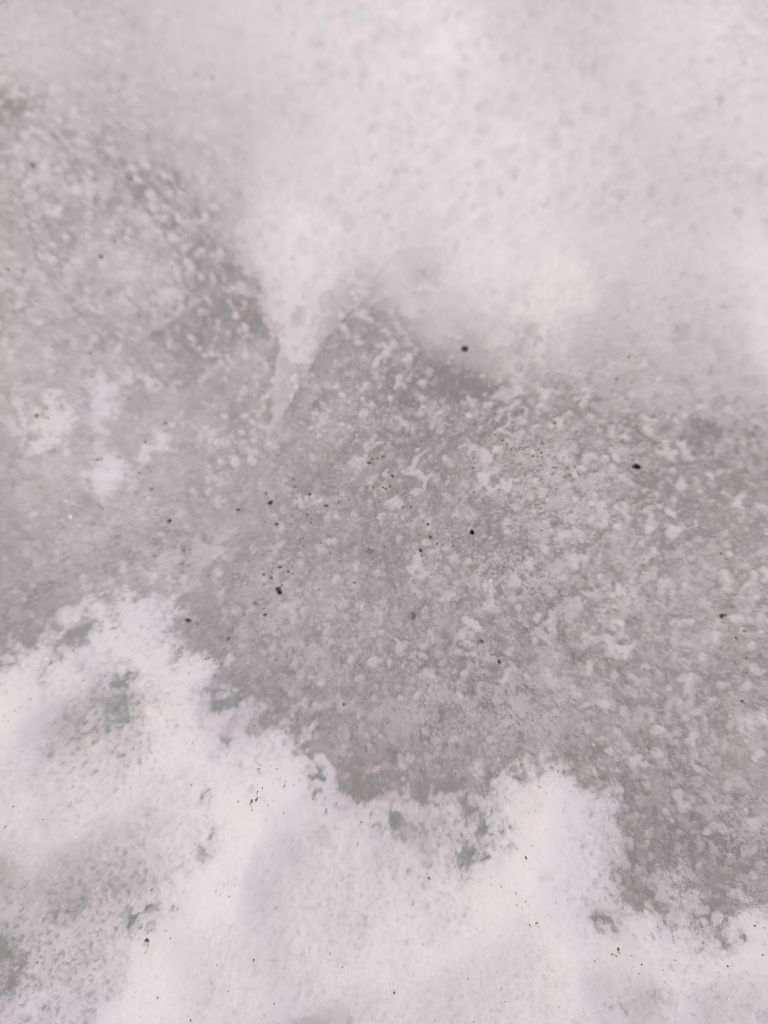
Darker glacier ice and lighter snow on a nunatak in Antarctica (photo: Ruth Mottram)

There’s an important feedback here too: melting darkens the surface, a darker surface absorbs more sunlight, and that helps even more melting. This is the albedo feedback and it’s a really important element in understanding how ice sheets will change in a warming climate. Each model has its own representation of the firn, and the melt albedo feedback and those details, multiplied over a century, produce completely different futures for the ice shelves.
The awkward bit is that our model is the pessimist of the bunch. HIRHAM simulates melt and refreezing rates today that are several times higher than MAR and RACMO, and it overestimates the number of melt days when compared with satellites. So when HIRHAM tells you the ice shelves are in trouble by 2100, it’s worth remembering that it’s the drama queen of the ensemble (there is nothing quite like co-authoring a paper that gently suggests your own model is the least well-behaved one). We’re pretty sure we know why: this version of the model has an albedo tuned for Greenland – too low for Antarctica and perhaps also some issues in the clouds.
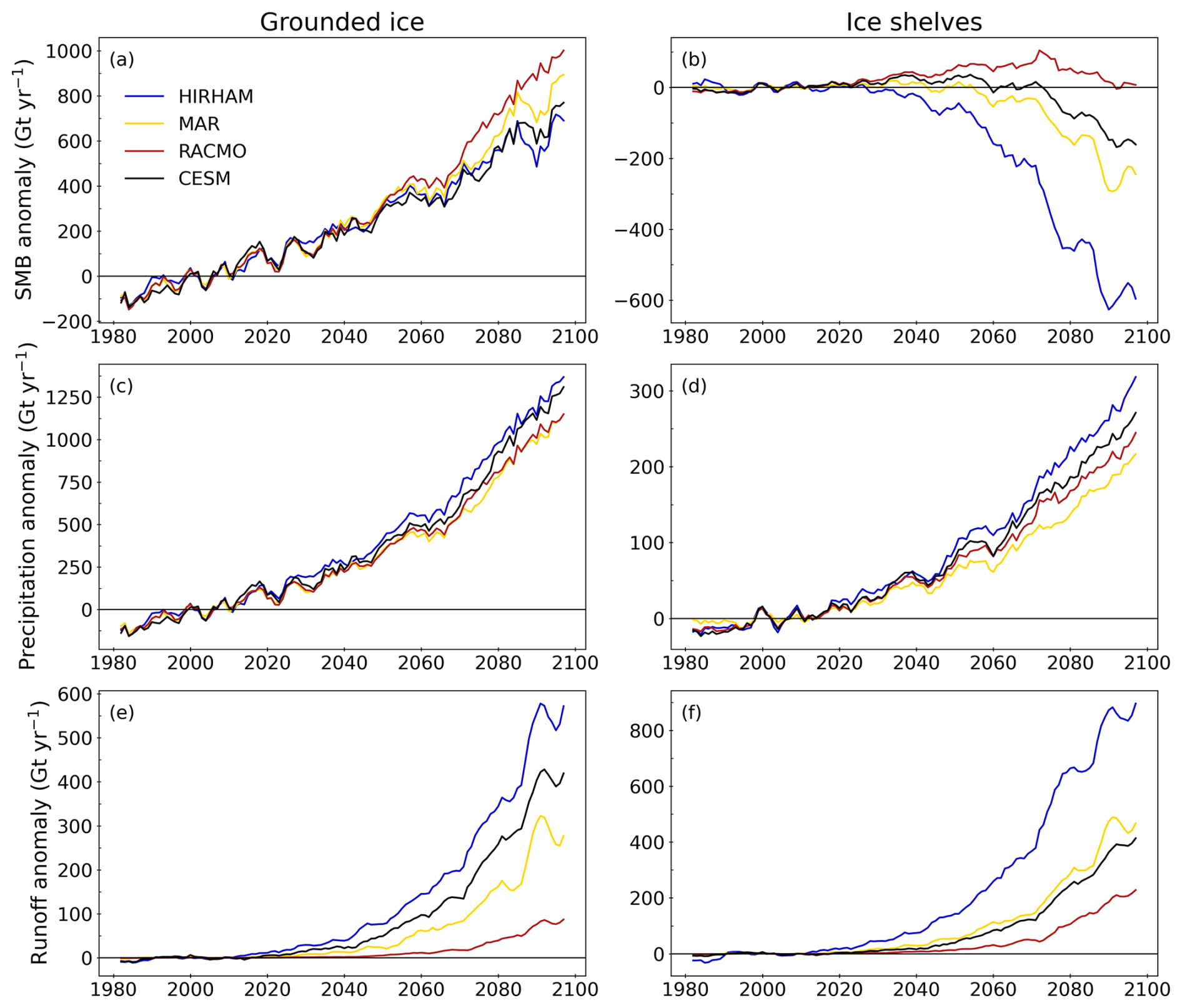
Figure 4 from the paper: Time series anomalies of SMB (a, b), precipitation (c, d), and runoff (e, f), in Gt yr−1, relative to the reference period 1995–2014. For the models MAR (yellow), HIRHAM (blue), and RACMO (red), driven by CESM2 (black) under the SSP5-8.5 scenario. Values are integrated over the grounded (left) and floating (right) parts of the Antarctic ice sheet. Note that the y axis scales differ between grounded and floating ice due to the difference in surface areas. A 5-year running mean is applied for clarity.

Interestingly though, even the two models that agree better with SMB at the start of the simulations, also diverge, as we also found in Greenland. The forcing model CESM2 also acquits itself respectably, though we have another couple of papers in the pipeline that muddy that picture a bit too..

The paper’s real point is that models agreeing on today’s climate does not guarantee they agree on the future — which matters a lot if you’re planning coastal defences, and argues for some hefty improvements in our understanding of the processes that happen at the interface of ice sheet and atmosphere. More on that soon too.


This paper originated with PROTECT, the EU Horizon 2020 project on projecting the ice sheet contribution to sea level rise, which for us at DMI wrapped up last year. Along with the multimodel projection datasets we produced for it, this feels like a good full stop on that project scientifically, though the projections will be included in planning for many years to come.


But there is another reason this feels like an ending: HIRHAM5, DMI’s polar regional climate model, has been retired for a few years now, and we’ve moved on to HCLIM, the climate version of the HARMONIE-ALADIN weather forecasting model.


This is, therefore very nearly the last HIRHAM paper. It will live on a little longer as the training data used in the development of our machine-learning model emulators, though there too we will soon switch to HCLIM (more on that another time), but as a model, HIRHAM is now in effect done.

“Finally, we would like to note that after 30 years of service the HIRHAM5 model was retired shortly after these simulations were complete, to be replaced by the HARMONIE-Climate system model (e.g. Verro et al., 2025). These will therefore be the last results published from HIRHAM, but the analysis here shows how important continuous assessment, improvement, development and evaluation of regional climate models is.”


Goodnight, sweet model.

As always, comments are welcome here, or find me on mastodon (@Ruth_Mottram).

Heurgue, B., Amory, C., Kittel, C., Boberg, F., Durand, G., Favier, V., Fettweis, X., Glaude, Q., Goelzer, H., Hansen, N., Jourdain, N. C., Mottram, R., Olesen, M., Van de Berg, W. J., Van den Broeke, M. R., and Wijngaard, R. R.:
Diverging runoff drives uncertainty in Antarctic surface mass balance projections under a high emission scenario, The Cryosphere, 20, 6353, https://doi.org/10.5194/tc-20-6353-2026, 2026.

Thirty years of hurt (and eleven years of writing about it) …


Every September, as the melt season on the Greenland ice sheet fizzles out, I and my colleague Martin Stendel do the same thing: we sit down with a year’s worth of daily surface mass balance maps and weather charts from the Polar Portal, work out how the ice sheet fared, and write it up as a guest post for Carbon Brief. Our latest one, covering September 2025 to August 2026 has just appeared over there (yes it’s a little late, we have a lot on right now).

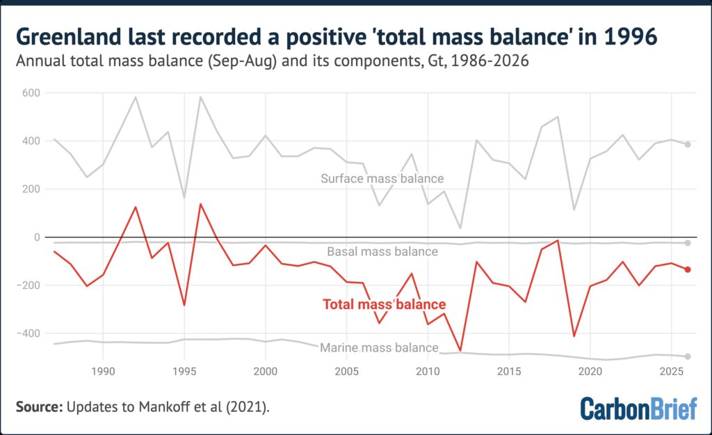
This year’s headline is one I’d rather not be celebrating: 2025-26 was the 30th consecutive year that Greenland lost more ice than it gained. The last year the ice sheet ended in the black was 1996. Even in a year with a cool, cloudy June, a late start to the melt season, and an above-average snowfall budget, it still lost around 135bn tonnes of ice.

The total mass budget of the Greenland ice sheet showing components from the surface, basal and marine budgets.


It struck me, reading back through copy number eleven, that we’ve now been doing this annual health check for over a decade, (we have been doing the famous Carbon Brief pub quiz for almost as long). And I think it’s time to look back and draw a few longer term lessons beyond the single year reports.

Why do we write them at all?

The honest answer is that a single year tells you almost nothing. In 2017 we reported a year where Greenland probably almost gained a small amount of ice — a one-year blip, thanks mostly to heavy snow delivered by the remnants of Hurricane Nicole from the Gulf of Mexico (weather is a long distance phenomenon, and Greenland gets its winter snow from some surprising places). In 2019 the ice sheet lost 329 Gigatonnes after a dry winter and a hot summer. In 2022 and 2024 it lost barely 80 Gigatonnes each. The weather in any given year can swing the budget by hundreds of Gigatonnes.

So while the annual posts are really about that specific year, they’re also a ritual: an agreed moment to check the patient’s pulse and write it down, in the same way, every year, so the numbers can be compared over the longer term. The point of the series is the series.


The baseline has shifted:

In 2021 I noted something that has stuck with me: that year’s surface mass balance, about 396 Gigatonnes, was thoroughly average for the current climate — but in the late 1990s the same number would have been one of the very lowest years on record. What counts as “normal” for Greenland now would have been an alarming outlier when I started. Shifting baseline as the biologists call it is real, but also for the physical climate system: we keep having to re-define “normal”, and in the case of mass budget it seems it is mostly downwards, but we also have to look back and remind ourselves regularly what normal was, back in the day.

When I was a child growing up in England, butterflies were common in our garden, our cars were often covered in dead insects, a hot summer day was 25C (very rarely 30C) and vast rivers of ice came plunging off alpine mountains. None of those things are true anymore.

The Greenland ice sheet is still a vast amount of frozen water, and it will take a very long time indeed for that to change, but the point of our annual health check is to detect, are there important changes in the stability of the patient?

Now for the obligatory small print warning: A healthy surface is not necessarily a healthy ice sheet. Every year, the surface mass balance defined as the snowfall in and the meltwater runoff (that is surface melt but minus any refrozen or retained in the surface snowpack)  out, just like in a bank account has been positive. Often comfortably above average. So far so good. 

But then every year for thirty years, the ice sheet has still shrunk, because the losses at the edges (icebergs calving, warm seawater melting glacier fronts) have quietly exceeded the surplus. I have lost count of the years where the headline was “good snow year, we still lost ice” including this year, where for example the Petermann glacier calved off a 76 km² ice island in early August regardless of the mild summer.

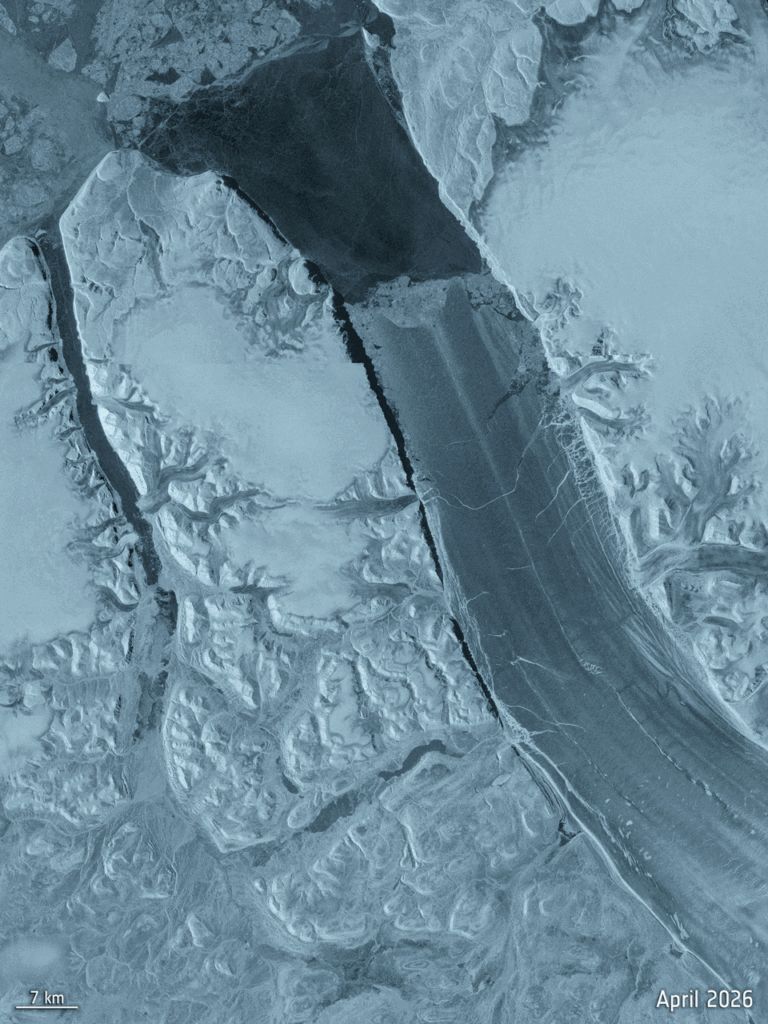
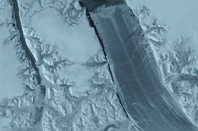
The Peterman Glacier prior to calving in April.

The surface is my own specialty, and I’m very fond of it, but it isn’t where most of the loss is coming from yet.

Through all of the series though, we can discern some consistent patterns. A dry winter plus a hot summer is the disaster recipe: as it was in 2019. A cool, snowy June acts like a shiny protective blanket and can rescue a mediocre year: 2021, 2023 and again this year. And remarkably often, while Europe and North America swelter in heatwaves, Greenland sits on the cool, wet side of the same stuck jet stream pattern. In 2018, 2023 and again in 2026 the same blocked “Omega” weather that baked Europe left Greenland comparatively damp and comfortable. The same pattern shifted by just half a wavelength in the atmosphere either way, and we’d be reporting record melt in Greenland instead.

Even the “nothing happened” years have been hiding things. In 2016 the year looked textbook average, until an April heatwave produced the earliest melt event on record, followed three months later by a new *cold* record in July. Average years, it turns out, are rarely average; you just have to look closely enough. (That year also taught me something about my own work: when we upgraded the DMI model, “average 2016” turned out to have been a rather low, unusual year. The instruments improve too.)

Taking the long view..

Earlier this year also saw publication of a big review I’m a (very minor!) co-author on, led by Prof. Edward Hanna at University of Lincoln, which synthesises everything we know about Greenland surface melt from 1500 CE out to 2200 covering data from ice cores, the satellite era and projections. It makes the same point out eleven annual posts have been circling around, but with 500 years of evidence instead of a decade: the year-to-year wobbles sum up to a trend that only points one way, and melt  is now visibly in the driver’s seat.


Thirty years is also a meaningful number for a different reason: it’s the length of a “climate normal” period the span climatologists use to separate a genuine shift in climate from natural variability. With 30 consecutive years of losses, warm years, cold years, snowy years, altogether we can now say confidently that what we’ve been writing in these annual posts isn’t weather any more. It’s climate change.

The long view: Hanna, E., Box, J.E., Fettweis, X., van den Broeke, M.R., Wake, L., Luu, L., Maddison, J., Mote, T., Mottram, R., Noël, B., Preece, J., Topál, D., Trusel, L. et al. Past, present and future Greenland Ice Sheet surface melt, 1500–2200 CE. Nature Reviews Earth & Environment, 7, 511–527 (2026) doi:10.1038/s43017-026-00800-3

The annual summaries are built on the daily monitoring at the Polar Portal supported by the Danish Meteorological Institute (through NCKF) and ESA’s Climate Change Initiative.

As always, questions and comments welcome below or on Mastodon

Meeting LISA

LISA: the Lightweight In Situ Analysis box is one of a kind; built by our friends at PICE in the Niels Bohr Institute. Later this year we’re taking LISA to Antarctica for the first time ever, to analyse shallow snow and firn cores directly in the field.

This is part of our contribution to the EPIC iQ2300 – a project led by Prof. Arjen Stroeven in Stockholm and organised by the Swedish Polar Research Secretariat.

iQ2300 is a huge project, and we are just a small part of it: the aim is to understand Dronning Maud Land’s evolution from the Holocene and out to 2300. Expect to hear a lot more about this effort in coming months…

Map of Antarctica, I lifted from polar.se : LISA will be visiting the Swedish Wasa station in DML – the top bit on this map – with us


Now back to our humble friend.

We hope LISA will help us understand how much snow falls in Dronning Maud Land, how much it varies from year to year and what is the influence of sea ice and far field atmospheric processes on the rate of snowfall. Snowfall is exceptionally difficult to measure and one of our biggest uncertainties in working out Antarctic mass budget and the response of Antarctica to a changing climate (spoiler alert: we might have a paper coming out about this shortly)…

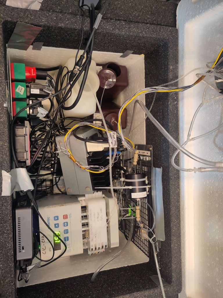
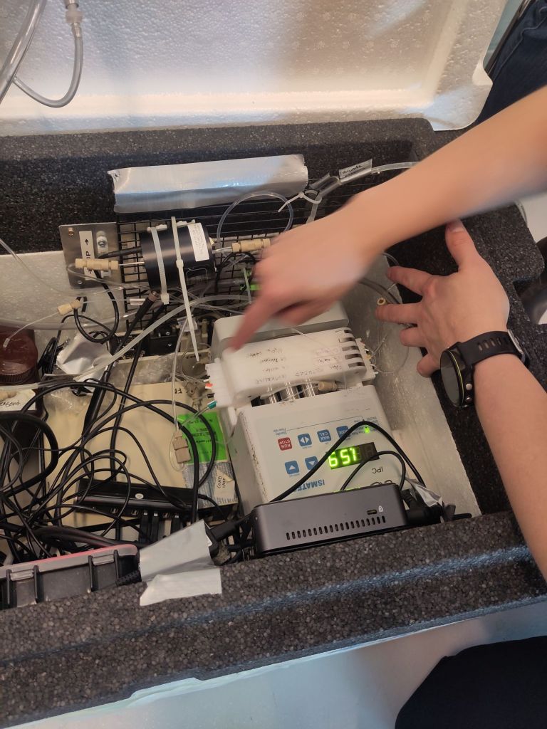
Meet LISA: a view inside the Magic Box..


Although LISA has been used in Greenland before, this is quite an experimental deployment, which means potentially really a lot of valuable scientific results. We would ultimately liek to build an Antarctic specific box, but that will have to wait to see if the results of this deployment are as good as we hope. (And some funding – if you are a billionaire with a spare couple of hundred thousand Euros, we’re always interested in talking).

The box itself is conceptually simple but in practice a little complex with a multiplicity of tubes, connectors and spare parts. This means it’s easy to fix if it breaks down, but also we need to understand how it works first.

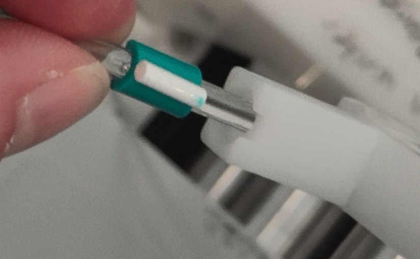
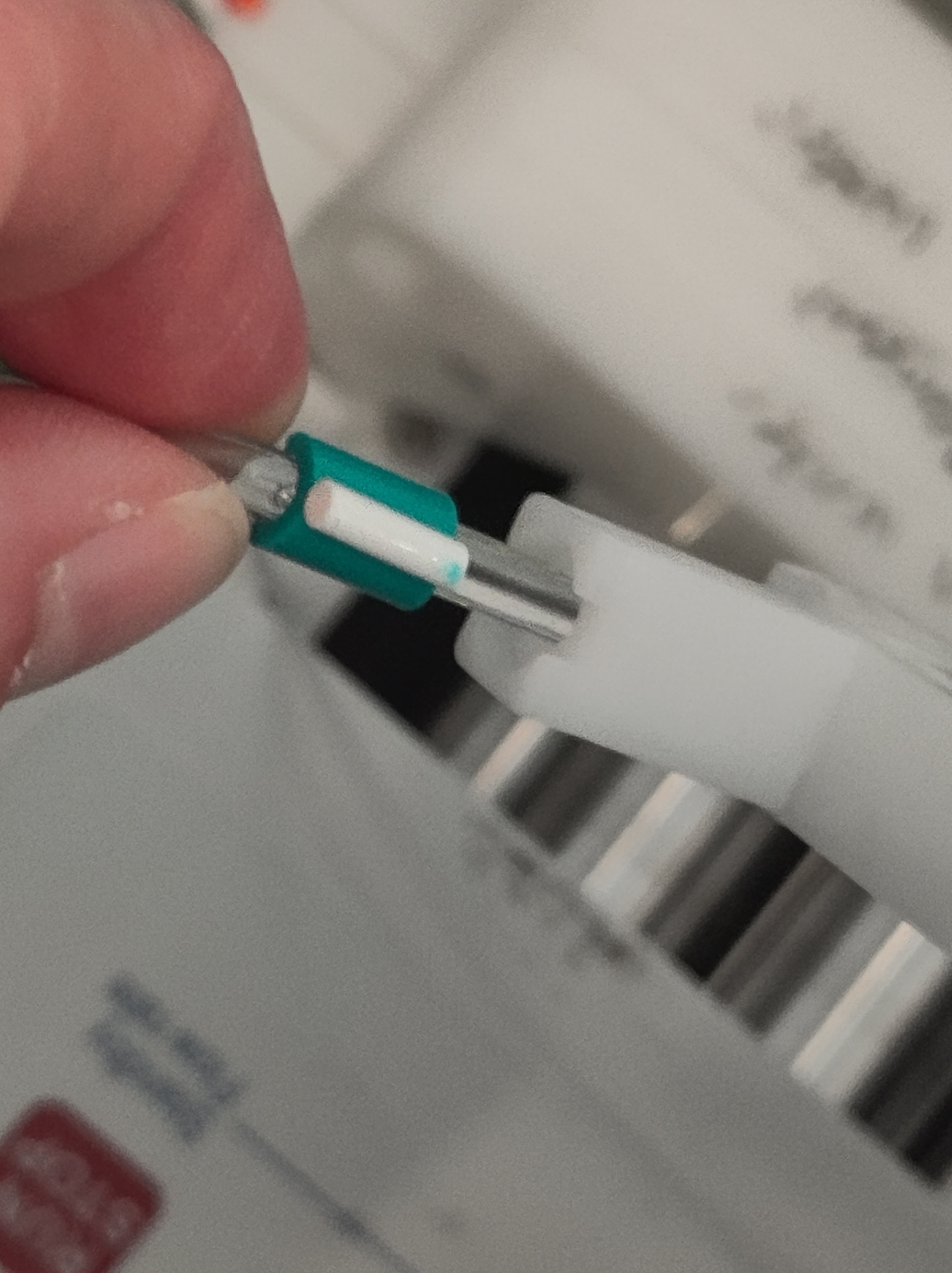
Some parts of LISA are quite fiddly…


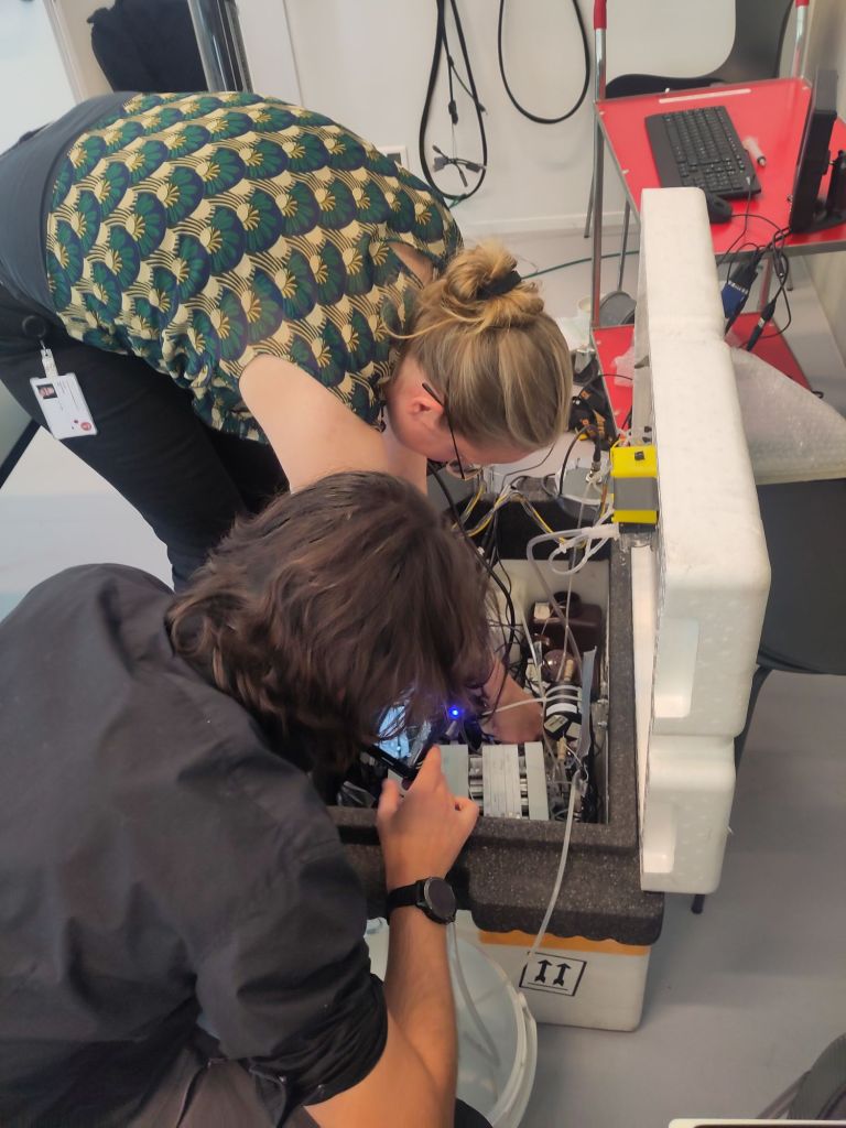
Today, the awesome and exceptionally generous Associate Professor Helle Kjær took myself, Stockholm Uni Prof Ninis Rosqvist and our PhD colleague from the Novo Nordisk funded PRECISE project, Clément Cherblanc through the use of the box.

Helle showing Clément the workings inside LISA

There’s a lot to remember and a lot to check but we’re reasonably hopeful we’ll get good results. The aim is to understand both the interannual variability on decadal timescales and the spatial gradients in snowfall accumulation. It’s a huge task, so it’s probably fortunate that we have 6 weeks or so (depending on the weather always!) to try and get it deployed at anumber of different sites which will hopefully allow us to do this.

It’s a big change to my normal fieldwork activities, but also a logical extension of them. And highly complementary to the climate and SMB modelling we are developing.

Nonetheless, ithere’s a lot of new stuff and I have in the past weeks learnt a great deal about transporting very small amounts of mildly hazardous chemicals on airlines, how to deal with customs and pack fragile instruments in large boxes.

Much more to come on this project, so stay tuned…

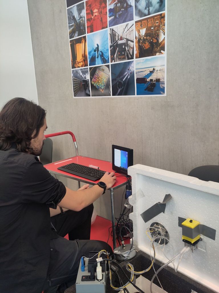
Clement getting stuck into using the software that measures different properties in the cores.

#PolarSekretariatet #AntarcticFieldwork #IceClimate #PolarClimate #Snow #SMB #AtmosphericVariability #iceCores #FirnCores #SnowCores

Small differences that make a really big difference.

I’m a co-author on a new paper that has just come out in GRL. It’s based on simulations we did with our collaborators in the PROTECT project on sea level contributions from the cryosphere.  What Glaude et al shows is that, to quote the first of the 3 key points:

“With identical forcing, Greenland Ice Sheet surface mass balance from 3 regional climate models shows a two-fold difference by 2100”

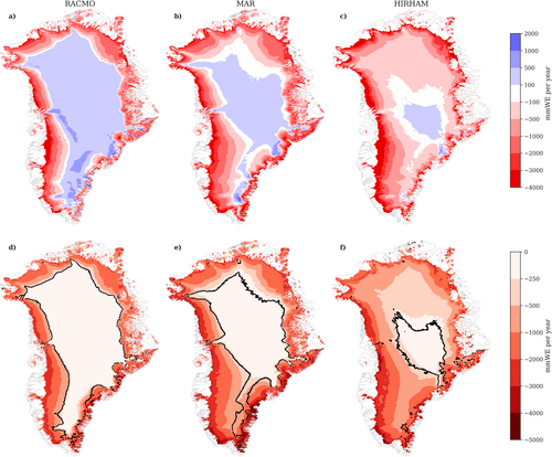
In perhaps more familiar terms, if you run 3 regional climate models (that is a climate model run only over a small part of the world, in this case Greenland) with identical data feeding in from the same global climate model around the edges, you will get 3 quite different futures. Below you can see how the 3 different models think the ice sheet will look on average between 2080 and 2100. The model on the right, HIRHAM5 is our old and now retired RCM. It has a much smaller accumulation area left by the end of the century than the other two, which have much more intense melt going on in the margins.

Greenland Ice Sheet annual surface mass balance (a, b, c, 2080–2099 average) and annual surface mass balance anomaly (d, e, f, 2080–2099 average relative to 1980–1999) [mm WE/yr]. From left to right, RACMO (a and d), MAR (b and e), and HIRHAM (c and f). The equilibrium line (SMB = 0) is displayed as a solid black line in (d-f). Glaude et al., 2024, GRL.

In fact, by the end of the century, although the maps above seem to show HIRHAM having much more melt, there is in fact more runoff from the MAR model, because of this intense melt.

Spatially aggregated annual GrIS SMB anomalies (a), total precipitation (PP, b), and runoff (RU, c) [Gt/yr]. The solid lines represent the anomalies using a 5-year moving average, while the transparent lines display the unfiltered model output.

The surface mass balance (SMB) at the present day is in fact positive. This often surprises people, but SMB as the name suggests, only describes surface processes. Ice sheets can (and do) also lose a lot of ice by calving and subglacial and submarine melt. As SMB should balance everything if a glacier is to remain stable or even grow, present day SMB is usually 300 to 400 GT positive at the end of each year, and even so the Greenland ice sheet loses, net around 270Gt per year.

Our work here shows that, at least under this pathway, not only does SMB become net negative in itself by the middle of this century, there are significant differences in SMB projections between the estimates of how negative it will be, between the three RCMs. The global model we used, CESM2 under the high-end SSP5-8.5 scenario, is famously a warm scenario, but our estimated end of the century SMBs are extraordinary : (−964, −1735, and −1698 Gt per year, respectively, for 2080–2099). As I’ve discussed previously, one gigatonne is a cubic kilometre of water, 360Gt is roughly 1mm global mean sea level rise. (Though note your local sea level rise is *definitely* not the same as global average!) Even the lowest estimate here the  is giving around 3 mm of global average sea level rise from surface melt and runoff *alone* by the end of this century each year. That’s pretty close to the modern day observed sea level rise from all sources.

And this is in spite of the fact that at the present day, the 3 models are rather similar in their estimates of SMB. The Devil is as usual in the details.

We attribute these startling divergences in the end of the century results to small differences in 1) the way melt water is generated, due to the albedo scheme (that is how the ice sheet surface reflects incoming energy); 2) but also due to the cloud parameters that control long-wave radiation at the surface, which again can promote or suppress melting. (We really need to know how much liquid water or ice there are in clouds, as this paper also emphasises in Antarctica); and 3) mainly down to the way liquid water that percolates down from the surface is handled in the snow pack. That is, how much air there is in the snowpack, how warm the snow is and how much refreezing can occur to buffer that melt.

The problem is that all of these processes happen at very small scales, from the mm (snow grains and air content), to the micron scale (cloud microphysics). That means that even in high (~5km) resolution regional models, we need to use parameterisations (approximations that generalise small scale processes over larger spatial and/or time scales). Small differences between these parameterisations add up over many decades.  Essentially,  much like the famous butterfly flapping its wings in Panama and causing a hurricane in Florida, the way mixed phase clouds produce a mix of water vapour and ice over an ice surface might ultimately determine how fast Miami will sink beneath the waves.

More data would certainly help to refine these parameterisations. The main scheme to work out how much liquid can percolate into snow was originally based on work by the US Army engineers in the 1970s. More field data with different types of snow would surely help refine these. Satellite data will be massively helpful, if we can smoothe out some wrinkles in how clouds (there they are again) affect surface reflectivity.

These 3 different types of processes also interact with each other in quite complex ways and ultimately affect how much runoff is generated as well as the size of the runoff zone in each model. So integration of many different types of observations is crucial.

“Different runoff projections stem from substantial discrepancies in projected ablation zone expansion, and reciprocally” as we put it in Glaude et al., 2024.

The timing and magnitude of the expansion of the runoff zone is quite different between the models, but all of them show a very consistent increase in melt and runoff over the next 80 years.

It’s probably also important to understand a couple of key points:

Firstly we ran a very high emissions pathway: SSP5-85 is probably not representative of the path we will follow in emissions (at least I hope not), but in this study we wanted to address the spread on different model estimates. And this is a way to get a good check on the sensitivity.

Secondly, the ice sheet mask and topography in these runs is kept fixed all the way through the century. This means we do not account for any elevation feedbacks (as the ice sheet gets lower because of melt, a larger area becomes vulnerable to melt because it’s lower and thus warmer), but we also don’t account for ice that has basically melted away no longer contributing to calculated runoff later in the century. Ice sheet dynamics are also not factored in.

Finally, we ran different resolution models, and that can have an impact particularly on precipitation and is one of the reasons why the new models we developed and have run in PolarRES (and which are now being analysed), have used a much more consistent set-up.

The 3 models we used, MAR, RACMO and HIRHAM have all been used in many different studies over both Greenland and Antarctica, but we haven’t really done a systematic comparison of future projections before. I think this work shows we need to get better at doing this to capture the uncertainty in the spread, especially when you consider that we’re now looking at using these models as training datasets for AI applications: training on each one of these models would give quite different results long-term. We need to think about how to both improve numerical models and capture that spread better. But ultimately, it’s how fast we can reduce greenhouse gas emissions and bend the carbon dioxide curve down that will determine how much of Greenland we will lose, and how quickly.

All data and model output from these simulations is available to download on our servers (we’re transitioning to a new one download.dmi.dk, not everything has been moved there yet). We also of course have data over land points and the surrounding seas, and we’ve run many more global climate models through the regional system to get high resolution (5km!) climate data also looking at different emissions pathways, if you’re interested in looking at, analysing or using any of this data – get in touch!

My warmest thanks to Quentin Glaude who led this analysis and special thanks to our colleagues in the Netherlands, France and Belgium for running these models and contributing to the paper analysis. Clearly, we have much work to do to get better at this ahead of CMIP7.

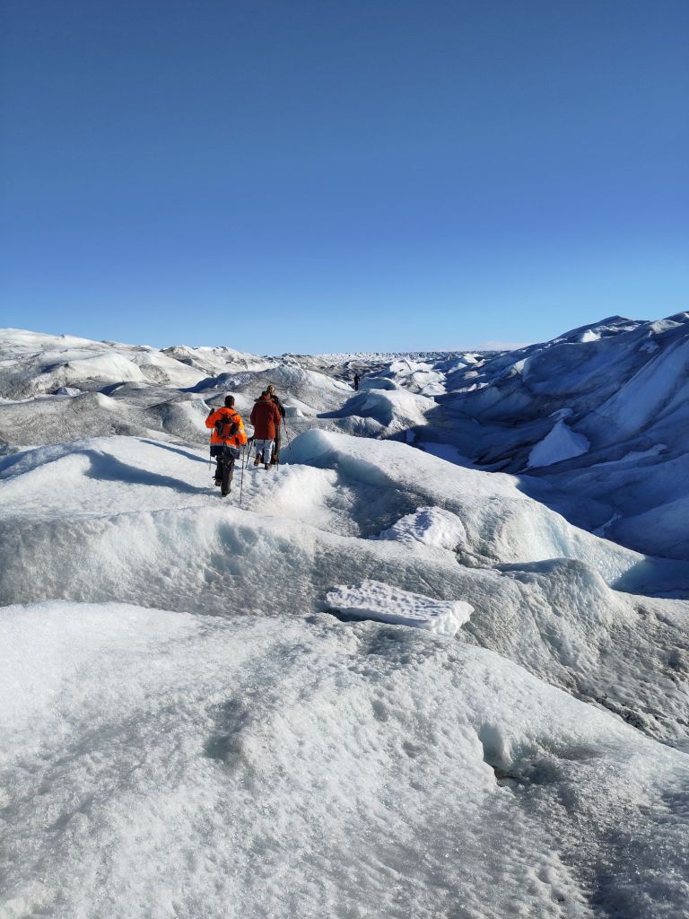
Group field trip the Greenland ice sheet: it’s important to see what you’re modelling actually looks like….