Half a century of ice loss: the new IMBIE dataset

More publication news! This month I’ve actually had 3 co-authored publications come out and hot on the heels of the mélange paper, a rather different piece of work I’ve contributed to has just come out: the latest assessment from the Ice Sheet Mass Balance Inter-comparison Exercise known as IMBIE to its friends, has just been published in Scientific Data. The paper is open access here: Otosaka et al., 2026. It’s the third (at least) in a series of articles monitoring the health of the ice sheets.
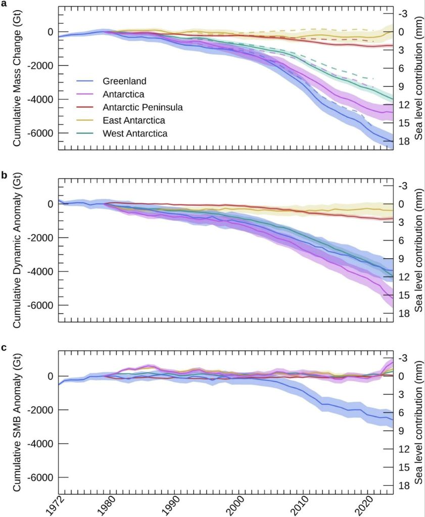
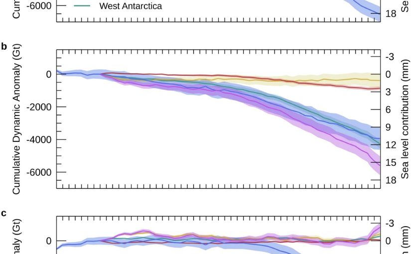
Figure 2 from the IMBIE paper is the money shot, as it were. The changes in ice sheet mass budget since the 1970s…

This one is a bit different from my usual, as it’s a data paper — the whole point is the dataset itself, which is freely available for anyone to download and use. But the numbers in it are rather striking and here is already a bit of misinformation spreading, so I thought it worth a short post.

What is IMBIE?

For readers who haven’t come across it before: IMBIE is a big international collaboration, supported by ESA and NASA, that tries to answer a seemingly simple question: how much ice are Greenland and Antarctica actually losing?

The problem is that measuring the mass of an ice sheet from space is really hard, and there are several different ways to do it — satellites that measure changes in ice sheet height (altimetry), satellites that measure changes in Earth’s gravity field (gravimetry), and the input-output method, where you compare how much snow falls on the ice sheet with how much ice flows out to sea at the glacier fronts. Each method has its strengths and weaknesses, and no single one gives the whole picture, specific choices in analysing satellite datasets can also give quite different results, not to mention model estimates of SMB can have a wide divergence.

IMBIE’s remit is to bring all the different groups together, get everyone to compute their estimates in a common framework, and then combine them. When many independent measurements agree, we can be much more confident in the answer, and that answer feeds directly into things like the IPCC reports and projections of future sea level rise. It’s community science at its best, even if it probably feels like herding cats to the fantastic coordinator Ones Otosaka, and I’ve been proud to contribute estimates from our HIRHAM5 surface mass balance modelling for both ice sheets to several of the IMBIE assessments over the years.

What’s new this time?

This latest assessment is the most comprehensive yet. The team combined 42 independent satellite surveys from 27 satellite missions — and extended the record further back than ever before, all the way to 1972 for Greenland and 1979 for Antarctica, using the early Landsat archive. That gives us a half-century view of how the ice sheets have changed. Though admittedly the recent years are much better covered than the earlier ones.

So what does half a century of satellite data tell us? (Note: just me who finds it hard to understand the 1970s as half a century ago?)

The two ice sheets have lost 11,300 billion tonnes of ice since 1979, raising global sea level by 31.4 mm — about three centimetres. Greenland accounts for the larger share, with Antarctica contributing 13.3 mm. The ice sheets are now responsible for roughly a quarter of all global sea level rise. The remainder is mostly due to thermal expansion as the oceans warms..

Three centimetres may not sound like much, but as Andrew Shepherd put it in the press release, that puts another six to nine million people at risk of coastal flooding and erosion. And the trend is very much in the wrong direction. In low-lying  Denmark this gives us more extreme storm surges and coastal flooding as even a few centimetres

A headline and a nuance: it’s the ice dynamics, not the surface melt, or is it?

There’s an important part of the paper which partitions the mass budget between dynamical losses and SMB changes. This is highlighted and the reasoning seemed obvious to me but in conversation with others is perhaps less obvious, so I want to discuss it here.

Of all that ice loss, 84% came from ice dynamics, that is outlet glaciers speeding up and discharging more ice into the ocean, from both calving icebergs and submarine melt, but “only” 16% from enhanced surface melting.

Now, I have spent a large part of my career working on surface mass balance, how much snow falls on the ice sheet and how much melts off it. We track it in near real-time on the Polar Portal, I write annual updates about it, and it’s genuinely important as it is the only way an ice sheet can maintain itself, no snowfall, no ice sheet.

Melt is also an important driver of ice dynamics, especially for Greenland. So it maybe should be with some professional humility that I report that the long-term mass loss story is apparently mostly a dynamics story: the ice sheets are responding to a warming ocean by flowing faster into the sea. Greenland’s rate of loss went from around 60 billion tonnes per year in the 1980s to 264 billion tonnes per year in the 2010s; Antarctica’s went from 48 to 202 billion tonnes per year over the same period, driven overwhelmingly by ocean melting at the outlet glaciers — with West Antarctica’s Pine Island and Thwaites glaciers leading the charge.

But there’s an important nuance in that 84/16 split, and it’s worth being clear about what it does and doesn’t mean. Surface mass balance is a two-way term: it’s positive when snow accumulates and negative when ice melts and runs off. And a warming climate pushes on both sides of the equation, more melt, certainly, but also more precipitation, at first as snow and increasingly we can measure over Greenland at least, as rain. Dynamic mass loss, by contrast, can only ever be negative: glaciers can only discharge ice into the ocean, they can’t drag it back up again. So we honestly wouldn’t expect SMB to be the biggest term in the loss budget, both sides of the SMB equation are increasing, it is in a race with itself. The genuinely worrying scenario is the one where melt and runoff together becomes bigger than snowfall. We are a very long way from that scenario fortunately, particularly in Antarctica but we’ll be in big trouble if, or perhaps when, that happens.

(Calving glaciology colleagues will note this whole discussion connects rather nicely to the question of what controls calving rates, which was the subject of my last post on melange…)

And now for a note of caution on the recent slowdown

You might have seen headlines suggesting ice loss has slowed down recently. It’s true that the most recent years in the record (2020–2023) show a temporary slowdown. A run of milder Greenland summers roughly halved its surface melting, and record snowfall over East Antarctica has offset some of the glacier losses there.

In fact we as a community have been on it as that East Antarctic snowfall is a story in itself. In a paper led by Marlen Kolbe earlier this year (Kolbe et al., 2026), (that I didn’t quite get around to talking about then, but I will rectify that), we showed that the extra snow is being delivered by atmospheric rivers — those great corridors of moisture streaming from a much warmer ocean towards the continent. Since 2020 they’ve become more frequent and more intense, dumping enough snow over East Antarctica to tip the whole ice sheet’s mass budget briefly into positive territory.

Is that reversal in mass budget temporary or permanent? Honestly, we don’t know yet but it matters because atmospheric rivers are double-edged. They bring massive snowfall, but they’re also often accompanied by a lot of melt — warm, wet air is rather good at melting ice as well as adding it. So the balance between accumulated snowfall and melt becomes more critical to understand here too, and the existing balance may well tip in the future.

The long-term picture remains one of accelerating loss, and as the climate continues to warm, we expect the losses to pick up again, especially in Greenland which is much further south than Antarctica is north, if that makes sense?
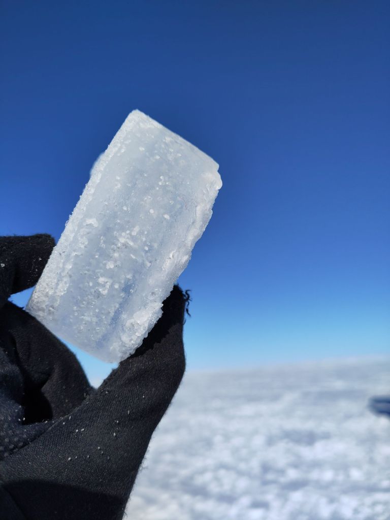
Refrozen melt layers in an Antarctic shallow ice core. We found a lot more of these than we expected based on satellites. Our all-seeing eyes in the sky don’t always see everything..

The response of the ice sheets to a warming climate is the single largest source of uncertainty in projections of future sea level rise. High-end estimates of global sea level rise by 2150 increase by a factor of 2.6 once the risk of ice sheet instability is accounted for. A continuous, half-century record of what the ice sheets are actually doing is exactly what we need to test the models and narrow those uncertainties, which is precisely why this dataset is such a valuable community resource, and why sustaining the satellite missions (CryoSat-2 and the Sentinels among them) that make it possible matters so much.

The full dataset is freely available from the UK Polar Data Centre, and you can read more about the IMBIE project at imbie.org. My thanks to Inès, Andrew, Tyler and the whole IMBIE team for pulling it all together — these assessments are an enormous amount of work, and the credit for this one belongs firmly with them.

As always, comments and questions welcome, here or on mastodon or blue sky.

Otosaka, I. N., Shepherd, A., Amory, C., et al. (2026). Mass balance of the Greenland and Antarctic ice sheets from the 1970s to 2023. Scientific Data, 13, 1301. https://doi.org/10.1038/s41597-026-08088-0
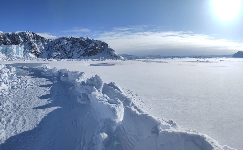
A jumble of broken ice, and what it means for Greenland’s calving glaciers.

Publication day! Our new paper has just come out in The Cryosphere, and after what feels like rather a long gestation, I’m delighted to finally be able to share it – The full paper is open access and available here: Hedetoft, Bang Brinck and Mottram et al. (2026).

This is the paper I was working on while I was in Ilulissat back in May 2024, watching icebergs drift around the bay and setting up time lapse cameras from my guest house window. At the time I wrote that “one of the papers I’m working on this week analyses those iceberg related datasets” — well, this is that paper, and it’s been quite a journey to get it into print.

The back story

As I wrote back in one of my several Qaanaaq posts, my colleague Steffen Malskær Olsen has been running a long-term observation programme in the fjord near Qaanaaq for 15 years now. That programme, and the field laboratory DMI maintains there, gave us an extraordinary opportunity to study something that glaciologists have been arguing about for years: what role does ice mélange actually play in controlling calving?

Ice mélange — sometimes known as sikussaq in Greenlandic — is that chaotic jumble of icebergs, bergy bits and sea water that sits in front of marine-terminating glaciers. It’s been described as the world’s largest granular material, and it’s a characteristic feature of pretty much every calving glacier in Greenland. In winter, landfast sea ice forms and acts as a kind of seasonal glue, sticking the whole mass together. The question is: does this frozen-together mass actually hold the glacier back, like a tiny ice shelf? Or is it more like a pile of rubble that the glacier shoves ahead of it with barely any resistance?

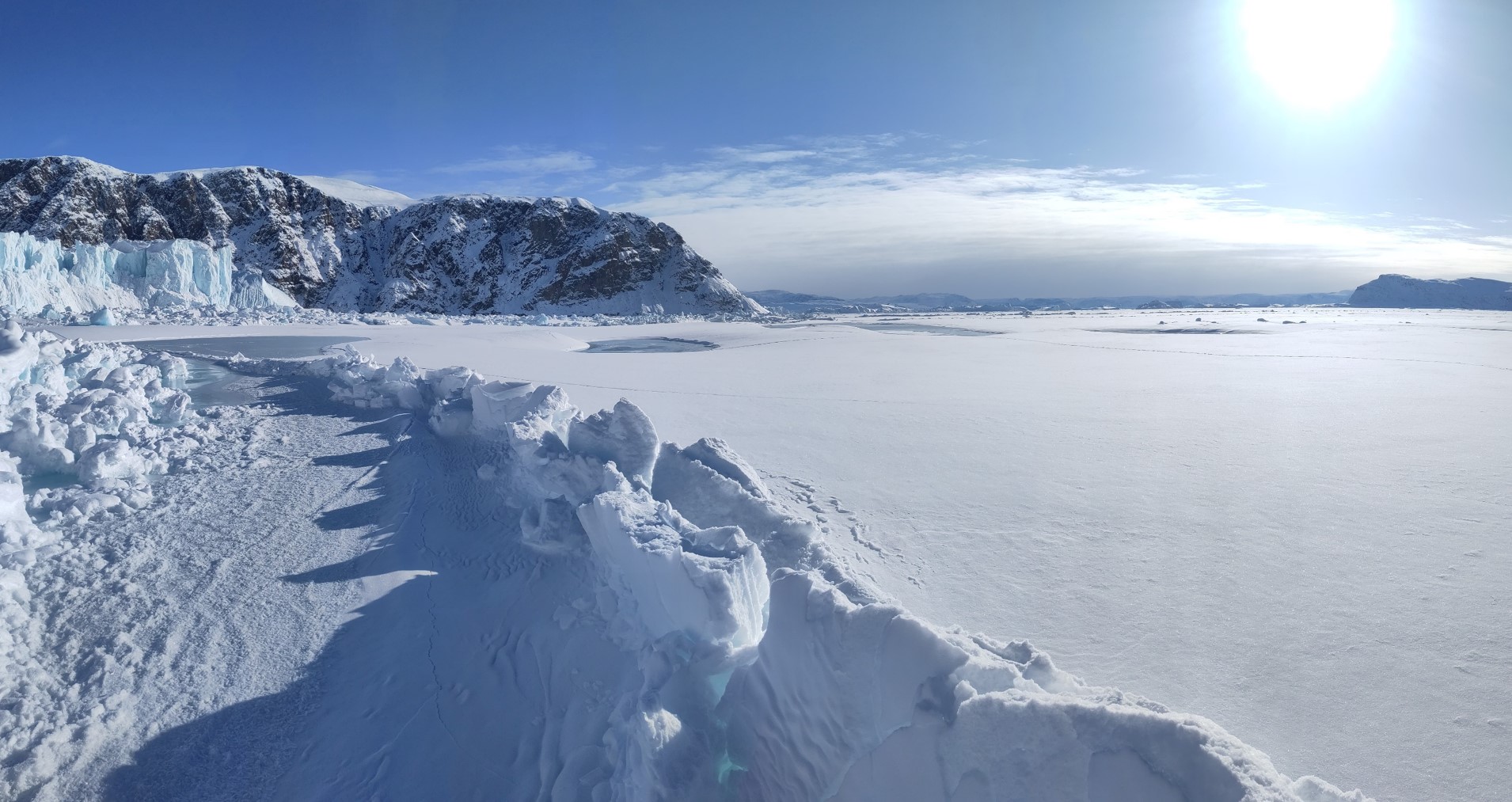
Iceberg melange in front of Melville glacier, with ridges and fractures in the sea ice forming as the glacier pushes through the winter.

The scientific community has been somewhat split on this. Some studies point to mélange as a mechanical inhibitor of calving — the idea being that calving only really kicks off once the mélange weakens or disappears. Others find the buttressing effect is limited, or depends heavily on whether landfast sea ice is present to bond the icebergs together. Most of the attention has been on the big, famous glaciers like Jakobshavn Isbræ and Helheim, which are enormous, fast-flowing, and in long narrow fjords. But what about the smaller, more typical glaciers that make up the majority of Greenland’s calving outlets?

That’s where Inglefield Fjord comes in.

The study site

We focused on three neighbouring glaciers at the head of Inglefield Bredning (Kangerlussuaq) in Northwest Greenland, at about 77.6°N: Tracy, Farquhar, and Melville glaciers. They’re a nice set because they’re different sizes — Tracy is the biggest at about 223 km², Melville is 119 km², and Farquhar is the smallest at 54 km² — and they’ve all been retreating at different rates over the last few decades. Tracy has been the fastest, retreating at about 200 m per year since the 1980s, twice as fast as Farquhar. Melville has been the slowest.

The area is also, crucially, accessible. The nearby town of Qaanaaq and the DMI field station there meant we could get out onto the sea ice by dog sled in late winter, working with local hunters and fishers who know the ice and the fjord far better than we ever will. This is something I want to emphasise, as I have before: this kind of science is a team sport, and the local community in Qaanaaq are absolutely essential to it.

What we did

The core of the study is a set of GNSS-tracking buoys that we deployed directly into the mélange zone, drilling holes in the sea ice and dropping them in. They recorded their position every 10 to 30 minutes and transmitted it back to us via the Iridium satellite network. When the sea ice broke up in July, the buoys floated free and were recovered by boat — again, thanks to our friends in Qaanaaq — and redeployed the following year.

We used two types of buoy: the TRUSTED buoys, which are a proprietary system from a Danish company (very robust as demonstrated by the incredible twists the metal stakes had from being over ridden by icebergs, a long battery life, but unfortunately rather limited position precision), and the OMB buoys, which are open-source instruments that we could customise to record more frequently, though they unfortunately proved a bit more vulnerable in this environment. Both have their strengths, and using both gave us a nice combination of reliability and detail. Not in the paper but deployed this year was even a third type – so watch out for more coming from this programme…

In March 2022 we deployed 6 buoys at Tracy and Farquhar. In March 2023 we deployed 8 buoys (6 TRUSTED and 2 OMB) across all three glaciers. The buoys tracked the mélange from late winter through to the break-up in mid-July, giving us a continuous, high-resolution record of how the mélange was moving — something that satellites alone can’t provide at this temporal frequency.

On top of the buoy data, we used quite a few other techniques to build a story.

  • Satellite imagery from ESA’s Sentinel-1 (radar, works in the dark and through clouds) and Sentinel-2 and Landsat (optical) to track calving front positions and identify calving events. We used a deep learning dataset from our co-author Erik Loebel to automatically extract calving front positions, but we also spent a lot of time manually checking satellite images because, frankly, the automated method sometimes confused the mélange edge with the glacier front, on the other hand our results independently confirmed that on a seasonal scale, the machine learning calving front detection actually works quite well!
  • Ice velocity data from our colleagues at PROMICE, again using ESA’s Sentinel-1 product, which (handily for us) isn’t masked to the ice sheet only, so it includes velocities from the mélange zone too.
  • Climate data from CARRA (the Copernicus Arctic Regional Reanalysis, a very cool 2.5 km resolution climate reanalysis for the Arctic) for winds, and our trusty HIRHAM5 regional climate model for surface melt and runoff timing.

The idea was to bring all these different datasets together and see how calving, mélange movement, glacier velocity, sea ice, and surface mass budget all interact over the course of a season.

What we found

I’ll try to keep this readable, but there’s quite a lot of detail in the paper for those who want it, so here are our key findings

1. The mélange moves steadily — with sudden jumps

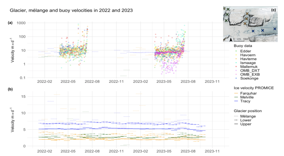
The buoys showed the mélange creeping slowly but continuously away from the glacier fronts, at speeds of roughly 2–11 metres per day, punctuated by occasional abrupt jumps. These jumps were larger and more frequent closer to the glacier fronts, and the larger Tracy glacier had more influence on mélange velocity than the other two. This fits with the idea of the glacier pushing the mélange down-fjord, like a slow-motion conveyor belt but with the rigid land fast ice causing resistance that abruptly fractures.

Velocity from the GNSS buoys at the top, compared with the satellite data at the bottom. The overpass and processing frequency of the satellite data smooths the velocities measured by the GNSS buoys.

2. Calving happens even in deep winter

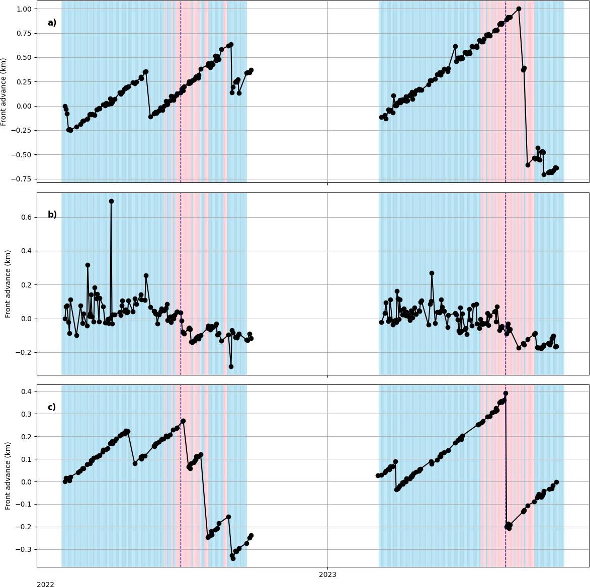
This was perhaps the most striking result. We observed large calving events at the peak of the fast ice season — in other words, when the landfast sea ice was at its thickest and most extensive, and the mélange was fully frozen together. Neither the landfast ice nor the mélange fully suppressed calving. This challenges the idea that mélange acts as a simple mechanical brake.

Calving front time series at the central flow line at (a) Tracy glacier, (b) Farquhar glacier and (c) Melville glacier for 2022 and
2023. Calving front positions are marked with black dots, and solid gray lines connect entries for each year. Red and blue backgrounds
symbolise positive and negative temperatures, respectively, based on 2m air temperature data from CARRA at 12:00UTC and the dashed
vertical lines represent sea ice break-up dates for the two years in question, 16 July 2022 and 25 July 2023, identified from changes in buoy
movements and examination of optical satellite imagery. (Loebel et al., 2023).

3. No tidal signal in the mélange

Inspired by this paper, we did a spectral analysis of the high-resolution OMB buoy data to look for tidal or diurnal cycles in the mélange movement. We found none. In fact we found something even a bit more interesting that – we had one buoy that seemed to show some kind of diurnal periodicity, but very complete spectral analysis found no tidal signal at all. We concluded the periodicity relates to the GNSS signal itself – a warning to analyse full all your data and consider other hypotheses as well as the favourite one!

The mélange during the fast ice season appears to be driven almost entirely by the glacier pushing from behind and perhaps by wind forcing, not by tides. This is interesting because tides are sometimes invoked as a driver of calving events via the melange, but at least at these glaciers during the fast ice season, we see no evidence of it.

4. Unbonded mélange doesn’t do much — it’s the landfast ice that matters – but only in winter

This is probably the key finding. When the mélange is just a loose jumble of icebergs (as it is in summer, after the sea ice has broken up), it has very little influence on glacier velocity or calving rates. It’s only when the individual ice blocks are frozen into a matrix of land fast sea ice — losing their “granular material” properties and becoming more like a rigid, multi-year sea ice cover — that they appear to exert any kind of braking effect. And even then, that effect is limited.

5. It’s a combination of factors

Putting it all together, our conclusion is that at these representative small and medium-sized Greenland outlet glaciers, seasonal calving behaviour is modulated by a combination of surface melt, glacier velocity, and the presence of landfast sea ice that bonds the mélange. It’s not one thing — it’s the interplay of several, and the landfast ice acts more to delay the removal of mélange than to prevent calving outright.

Why does this matter?

Calving processes account for roughly half of the total mass loss from the Greenland ice sheet, yet they remain poorly represented in ice sheet models. It’s something I’ve been working on since my PhD. If we can’t model calving properly, we can’t project future sea level rise properly — and for a country like Denmark, that’s a rather existential question.

Most previous mélange studies have focused on the big, dramatic glaciers. Our study suggests that at the more typical, smaller glaciers that make up the bulk of Greenland’s calving outlets, the story is more nuanced. Mélange buttressing isn’t a simple on/off switch. It depends on whether the icebergs are bonded together by landfast sea ice, and even then, the effect is modest. Surface melt and glacier dynamics seem to matter more and these are all inter-realted processes, typically the air temperature gets warmer, the ice surface starts to melt, the glacier starts to accelerate and the sea ice gets weaker and thinner all at the same time. We have confounding variables which makes the picture difficult to disentangle.

We also hope the dataset we’ve collected — the in-situ buoy tracks, the satellite-derived calving fronts, the velocity comparisons — will be useful for other groups working on modelling mélange processes. There’s very little in situ data across seasons with this kind of temporal resolution, and we’d be delighted if others can use it to test and improve their models.

Some Criticisms… and what’s next?

We had a very excellent editor and really good reviewers who gave the paper a through filleting. You can see these online as the Cryosphere has open review. I thank them all for their good comments which certainly clarified the paper. The main criticism that may still be levelled is what about the melange thickness? Maybe these glaciers don’t see an effect because the melange is thin and weak? Well we do go into that in the paper. These are pretty representative glaciers for Greenland by any measure and perhaps the glaciologists view of melange processes is slightly skewed by all the studies at Jakobshavn/Sermeq Kujalleq and Helheim? However, when you stand in the melange zone, it becomes very clear just how heterogenous it is. The large icebergs make up a relatively small portion of the total area, so current models, using “melange thickness” as a tuning parameter are missing some subtlty, which probably turns out to be important in this subject area.

And there’ll definitely be more on melange dimensions and how that relates to buttressing, coming very soon!

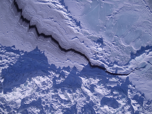
UAV shot of a sea ice lead in the melange zone of Tracy glacier, 2023

Acknowledgements

This paper was led by Sofie Hedetoft and Olivia Bang Brinck, who share first authorship with me and who did the lion’s share of the analysis and making of the figures. It’s been a real pleasure working with them and we would certainly not have got very far the rest of the team: Andrea Gierisch and Steffen Malskær Olsen, who were fantastic field work colleagues and a great inspiration for the ideas in this paper, Martin Olesen and Nicolaj Hansen for climate and SMB insights, Anders Anker Bjørk for finding our marvellous students and offering great advice on ice velocioty products, Erik Loebel for the automated calving front analysis, Anne Solgaard for the satellite data processing and assistance in interpretation and Peter Thejll whose expertise in statistics and spectral analysis is unrivalled.

As ever, none of this would have been possible without the local community in Qaanaaq — the hunters and fishers who guided us, transported us by dog sled, helped install instruments and recovered our buoys by boat when the ice broke up. Our DMI colleague Aksel Ascanius, who lives and works in Qaanaaq, has been an essential part of the programme throughout.

The work was carried out under the auspices of the Danish National Centre for Climate Research (NCKF), funded by the Danish Government, with additional contributions from EU Horizon Europe frameworks and ESA’s Climate Change Initiative for the Greenland ice sheet.

The full paper is open access — please go and read it, and do get in touch if you have questions or comments. I’m always happy to hear from people, whether on here, on mastodon, or by email.

Hedetoft, S., Bang Brinck, O., Mottram, R., et al. (2026). Mélange, landfast sea ice, ice velocities: What controls seasonal calving rates in North West Greenland? The Cryosphere, 20, 5071–5098. https://doi.org/10.5194/tc-20-5071-2026