
There is currently some discussion in the Danish media about sea level rise hazards and the risk of rapid changes that may or may not be on the horizon. Some of the discussion is about IPCC estimates. That’s a little unfortunate and in fact a bit unfair as the IPCC report has not been updated since 2021, nor was it intended to have been. In the mean time there has been a lot of additional science to clear up some of the ambiguities and questions left from the last report.
I’ve been working quite a bit on the cryosphere part of the sea level question of late, so thought I’d share some insights from the latest research into the debate at this point. And I have a pretty specific viewpoint here, because I’ve been working with the datasets, models, climate outputs etc that will likely go into the next IPCC report as part of a couple of EU funded projects. As part of that, we have prepared a policy briefing that will be presented to the European Parliament in June this year, but it’s already online now and will no doubt cross your socials later this week. I’m going to put in some highlights into this post too.
Now, I want to be really clear that everything I say in this post can be backed up with peer reviewed science, most of which has been published in the last 2 to 3 years. Let’s start with the summary:.:
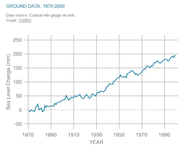
- The sea is rising. And the rate of rise is currently accelerating.
- The sea will continue to rise long into the future. The rate of that sea level rise is largely in our society’s hands, given that it is strongly related to greenhouse gas emissions.
- We have already committed to at least 2m of sea level rise by 2300.
- By the end of 2100 most small glaciers and ice caps will be gone, mountain glaciers will contribute 20-24% of total sea-level rise under varying emission scenarios.
- Antarctic and Greenland ice sheet mass loss will contribute significantly to sea-level rise for centuries, even under low emissions scenarios
- Abrupt sea level rise on the order of metres in a few decades is not credible given new understanding of key ice fracture and iceberg calving processes.
- By the end of this century we expect on the order of a half to one metre of sea level rise around Denmark, depending on emissions pathway. (If you want to get really specific: the low-likelihood high impact sea level rise scenario corresponds to about 0.9 m (on average), or at the 83rd percentile, about 1.6 m of sea level rise).
- Your local sea level rise is not the same as the global average and some areas, primarily those at lower latitudes will experience higher total sea level rise and earlier than in regions at higher latitudes.
- We have created a local sea level rise tool. You should still check your local coastal services provider, they will certainly have something tailor made for your local coastline (or they *should*!), but for something more updated than the IPCC, with latest SLR data, this is the one to check.

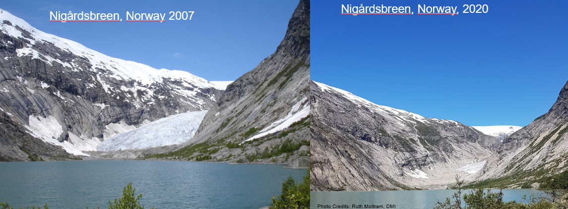
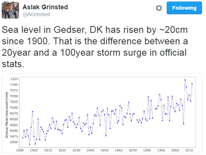
Sea level rise now is ~5mm per year averaged over the last 5 years, 10 years ago it was about 3 mm per year). Much of that sea level rise comes from melting ice, particularly the small glaciers and ice caps that are melting very fast indeed right now. Even under lower levels of emissions, those losses will increase. There won’t be many left by the end of this century.

Greenland is the largest single contributor and adds just less than a millimetre of sea level rise per year, with Antarctica contributing around a third of Greenland, primarily from the Amundsen Sea sector. The remaining sea level rise comes from thermal expansion of the oceans. Our work shows very clearly that the emissions pathway we follow as a human society will determine the ultimate sea level rise, but also how fast that will be achieved. The less we burn, the lower and slower the rise. But even under a low-end Paris scenario, we expect around 1 metre of sea level by 2300.

The long tail of sea level rise will come from Antarctica, where the ocean is accelerating melt of, in particular, West Antarctica. However, our recent work and that of other ice sheet groups shows that the risk of multi-metre sea level rise within a few decades is unrealistic. Again, to be very clear: We can’t rule out multiple metres of sea level rise, but it will happen on a timescale of centuries rather than years. High emissions pathways make multiple metres of sea level rise more likely. In fact, our results show that even under low emissions pathways, we may still be committed to losing some parts of especially West Antarctica, but it will still take a long-time for the Antarctic ice sheet to disintegrate. We have time to prepare our coastlines.

Greenland is losing ice much faster than Antarctica, and here atmospheric processes and firn and snow are more important than the ocean and these are also where the læarge uncertainties are. As I’ve written about before, that protective layer of compressed snow and ice will determine how quickly Greenland melts, as it is lost, the ice sheet will accelerate it’s contribution to sea level. This is a process that is included in our estimates.

There’s so much more I could write, but that’s supposed to be the high level summary. Feel free to shoot me questions in the comment feeds. I’ll do my best to answer them.
Five years ago, a small group of European scientists got together to do something really ambitious: work out how quickly and how far the sea will rise, both locally and on average worldwide, from the melting of glaciers and ice sheets. The PROTECT project was the first EU funded project in 10 years to really grapple with the state-of-the-art in ice sheet and glacier melt and the implications for sea level rise and to really seek to understand what is the problem, what are the uncertainties, what can we do about it.
We were and are a group of climate scientists, glaciologists, remote sensors, ice sheet modellers, atmospheric and ocean physicists, professors, statisticians, students, coastal adaptation specialists, social scientists and geodesists, stakeholders and policymakers. We’ve produced more than 155 scientific papers in the last 5 years (with more on the way) and now our findings are summarised in our new policy briefing for the European Parliament.
It’s been a formative, exhilarating and occasionally tough experience doing big science in the Horizon 2020 framework, but we’ve genuinely made some big steps forward, including new estimates of rates of ice sheet and glacier loss, a better understanding of some key processes, particularly calving and the influence of the ocean on the loss of ice shelves. More importantly for human societies, by integrating the social scientists into the project, we have had a very clear focus on how to consider sea level rise, not just as a scientific ice sheet process problem, but also how to integrate the findings into usable and workable information. In Denmark, we will start to use these inputs already in updating the Danish Climate Atlas. If you are elsewhere in the world, you may want to check out our sea level rise tool, that shows how the emissions pathway we follow, will affect your local sea level rise.
Our final recommendations?
- Accelerate emission reductions to follow the lower emission scenario to limit
cryosphere loss and associated sea-level rise - Enhance monitoring of glaciers and ice sheets to refine models and predictions
- Support the long-term development of ice sheet models, their integration into
climate models, and the coupling of glacier models with hydrological models, while
promoting education and training to build expertise in these areas - Invest in flexible and localized coastal management that incorporates
uncertainty and long-term projections - Foster international collaboration to share knowledge, resources, and strategies
for mitigating and adapting to global impacts


