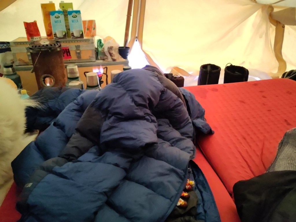
I very rarely have time to write a proper field diary, our time in the field is usually extremely hectic and filled with 12-18 hour working days that blend seamlessly together. I suspect this week is also going to be busy, but Nature has offered an olive branch in the shape of an early break-up of the sea ice, so I’m taking a moment to write a few things down. Updates will be posted at the top so scroll down to read the first day.
And finally…
I’m writing this on the metro home, I’ll spare you the flight delays, the packing up dramas, the last minute, “just one more snow pit”…

It was a good tour. Enormous amount of work done, perhaps more importantly, it has also been foundational work, on both data and field site management, it will be much easier for colleagues to help us maintain this and to build up a long term data set of all the observations (and more that I haven’t written about here) in future. That should reduce costs and field time in the future but also give others the opportunity to visit and do their own research up here.

I think streamlining the storage of data is extremely important. There is far too much data in the world on hard drives and in field notebooks, doing no good to anyone. This system will be much easier for other colleagues to use what we have collected and we will be able to publish them outside of DMI soon too. I remain committed to FAIR publishing, but I often feel the barriers are practical rather than psychological.
I’ve also introduced my new(ish) colleague Abraham to the Arctic. Given he grew up in a place without snow it has been a delight to watch him discover the processes and problems that I’ve been working on the last 20 years and that we’ve been discussing together the last 18 months. I believe it’s extremely important for climate modellers to understand and see the system they’re trying to model. This trip has definitely confirmed me in that. This was not just a field campaign but also a pedagogical field trip in some ways too. We have also had the opportunity to brainstorm a lot of new research ideas along the way, there is rarely such time in the office, so plenty more to work on in coming years..
As ever massive thanks to many colleagues, especially Aksel our DMI station manager without whom this work would be close to impossible given he is both interpreter and collaborator on the practical observations; Qillaq Danielsen for taking us out on to the sea ice with his sled. Steffen for running an extremely valuable long-term programme, Andrea for helpful and practical discussions and of course Abraham for making it a very good week. Glad we got to do this.
I should also say a large thankyou to my husband for keeping the home front running smoothly along whilst I am travelling. None of this would work otherwise.
Tak for denne gang Qaanaaq!
Day 6: Last day
It’s amazing how fast the tine goes, our last full day in the field (we’d originally planned for 9 days, but that was partly because last year we planned a week and it got cut to 3 days due to flight weather problems, I learned and left a safety margin this year). Nonetheless, a busy day. As we’re really interested in lots of different processes that combine in what we call the Arctic Earth System our focus for today was twofold, looking at the atmosphere and the subsurface, both of which are partly other scientists projects, but giving data we really want to use with our climate model, both for evaluation and development.

The main aim was to finalise the snow site ready for observations over the next year. We finally reinstalled the remaining FC4 and new logger, this has been ticking over and being tested in our station kitchen for the last couple of days. I’m rather pleased with myself in managing to get these 2 talking to each other, I was envisaging a bigger struggle, but the Campbell Scientific software is very easy to use with good user guides.
The installation was the last element for the snow site and after Aksel and Abraham’s sterling work in building our new logger station, it was trivially easy.

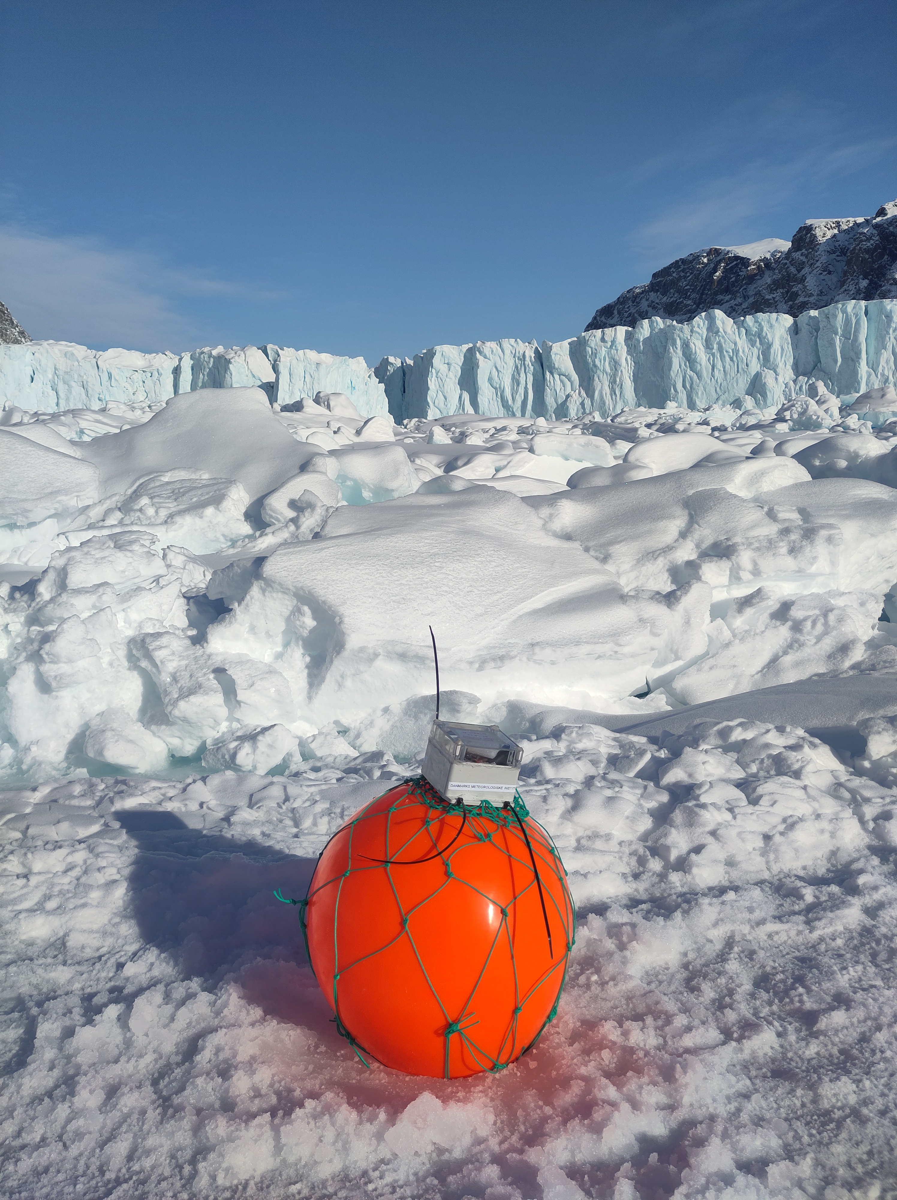
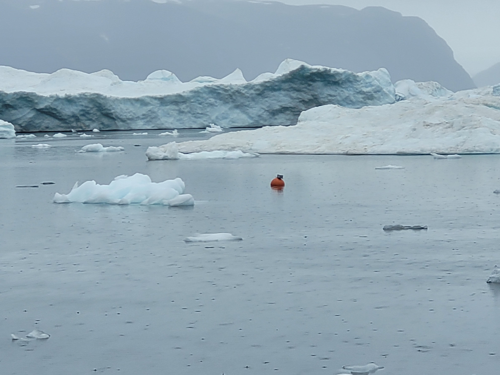
The experience with the new Campbell system proved invaluable in the next task, downloading a whole bunch of data from colleagues’ weather stations for shipping back to Denmark. Normally, we would have been a bigger crew to handle work on the sea ice as well as at the station, but as the sea ice broke up so early (see Day 1), our local hunter friends had taken them down and brought them in to Qaanaaq for us. They needed a bit of repacking, data downloads and checks and we set up a skin temperature calibration station for the satellite group, which I think will also be quite interesting for us in polar regional climate modelling to use. This we left overnight for longest possible calibration.
As we have many collaborations we also spent an hour trying to collect some data from the subsurface permafrost sensors installed by our colleagues at the University of Copenhagen. Unfortunately, it appears they need rather more maintenance than we can provide, so that will need a full team. I am extremely keen to see the data though, ten years + of permafrost and temperature measurements is a seldom dataset and will be super interesting to use in the further development of our surface scheme. Qaanaaq is somewhat vulnerable to permafrost disturbance as it is built on sediments, so monitoring this in a warming climate is pretty important.
A long day, but made even longer by the excitement of narwhals in the bay! We headed out to the ice edge at 11pm, (the polar day plays havoc with your body clock), where quite a few hunters had gathered and were busy slicing up a freshly caught narwhal, eagerly filmed by at least one of the several film crews and photographers there appear to be in the town right now. We have noticed increasing numbers of film crews visiting this part of the world. It can be surprisingly busy.
Greenland does have a strictly regulated quota on narwhals, it’s an important part of the culture, but it is a bit brutal to watch if you’re not used to seeing animals sliced up. Personally, I think everyone should see where the meat they eat comes from. It would make us all more honest about agriculture. But I digress, I was actually more excited to see live ones out in the bay. We’re immensely fortunate to see them, this is only the 2nd time in 5 years I have seen live narwhal here, and it’s only really because the ice has shrunk so early allowing them in. I have immense respect for the hunters who go out in flimsy lightweight kayaks to harpoon them. That must take some courage.

UPDATE: And as an aside, our ace colleagues and collaborators at the Greenland Institute of Natural Resources have a wonderful series of videos exploring all kinds of research in Greenland, including this brilliant one featuring Malene Simon Hegelund and my DMI colleague Steffen Olsen, together with Qillaq Danielsen who we were also out with this year, which really gives a flavour of fieldwork in Qaanaaq and just how important our collaborations with the local community and Greenlandic scientists are.
Day 5: Glacier Day!
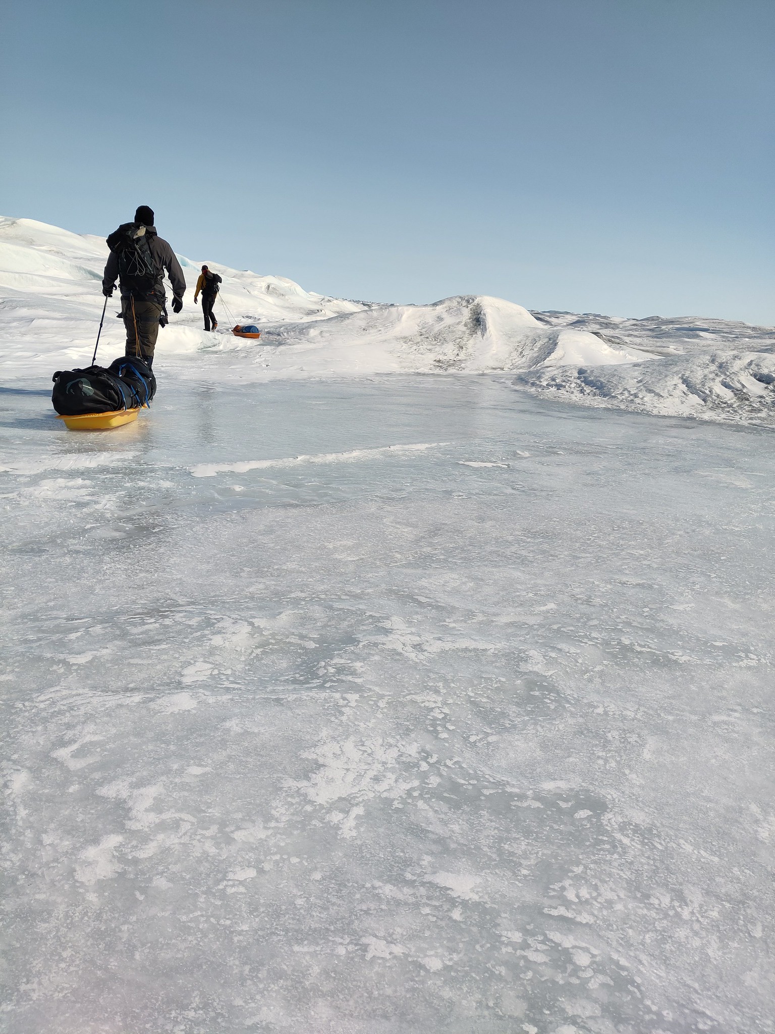
As an unrepentant glaciologist, I always look forward to glacier day, when we get up onto the land ice. In this case it’s only a tiny outlet glacier from a rather small local ice cap (well I say small, in the Alps it’d be considered quite large, but by Greenland standards it’s small but well studied). It’s easily accessible and the point about today was to take surface snow measurements and density profiles, so accessible is good.

The deep soft snow that has been a bit of a bane everywhere this year was also a problem. It was very heavy going, there isn’t really a path, just very loose rocks in a (at this time of year dry) riverbed, which is bad enough in summer but when covered in 30cm of snow was quite heavy going. Nonetheless we made a decent pace and got quite high up. By the time we came down again, the outwash river was starting to show signs of life again. It was a cold day, between -3 and -5C but the blazing sunshine alone is enough to start to generate melt and we saw plenty of signs of radiation driven melt going on under the surface snow crust, especially where there were dust layers to accelerate the process.
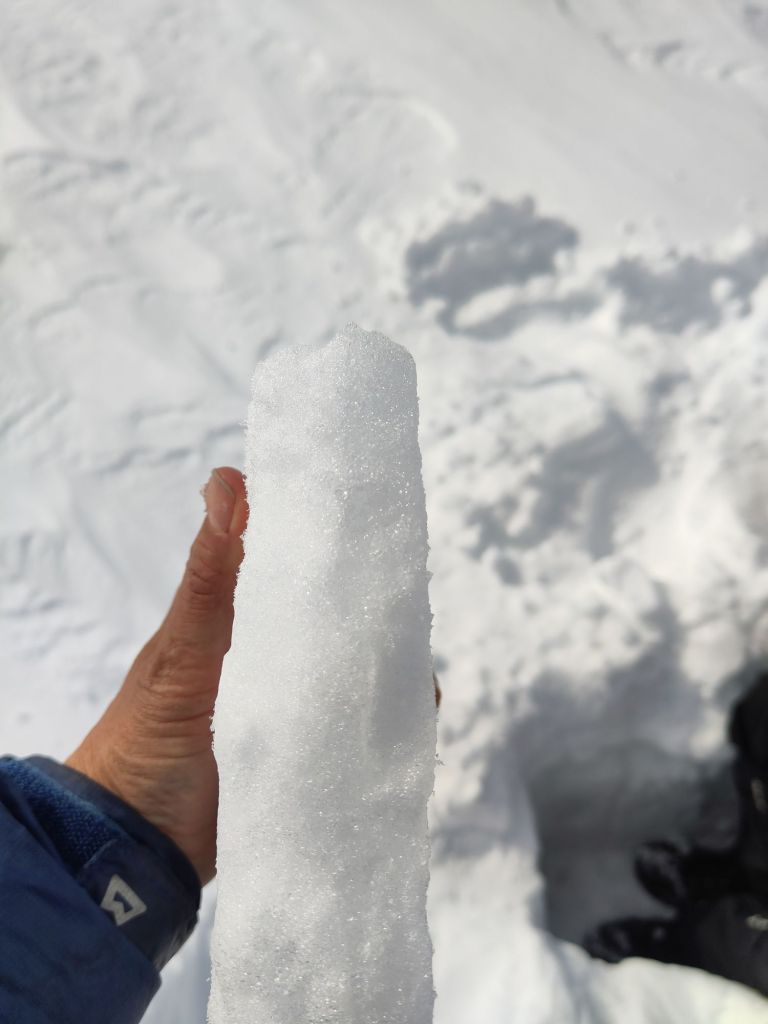
The snow pits proved indeed how cold the snow has been, typically around -10C at the bottom of the pits, but in one we also found signs of refrozen melt water, perhaps from the brief March warm period?

We did a transect down with our borrowed infrasnow, made several density profiles and had quite an efficient time. The idea is to repeat this transect at different times of the year so we can see how the snow properties change. In particular, I’m interested in surface albedo (how much incoming light is reflected by a surface). The reflectivity of the snow and ice surface is extremely important for the energy budget, which in turn controls how fast the snow (and ice) melt as well as being important for satellite data retrievals of surface temperature.
The Infrasnow is a very neat device that measures density and specific surface area. It’s not quite the same thing as albedo but it will help us to develop our albedo scheme in the model as it is based on grain size. Unfortunately it does not work on glacier ice, which is some places we also saw peeking out the top where wind has scoured the surface snow away. The movement of snow by wind is the subject of our final full day in the field.

We continued the observations off the glacier all the way to the road so we have a nice base transect that can be repeated to assess how conditions change through the year.
Although we only hiked 10km, it was quite tough, so next year we’ll bring snow shoes…
Tomorrow is our final full day. Lots more to do.
Day 4
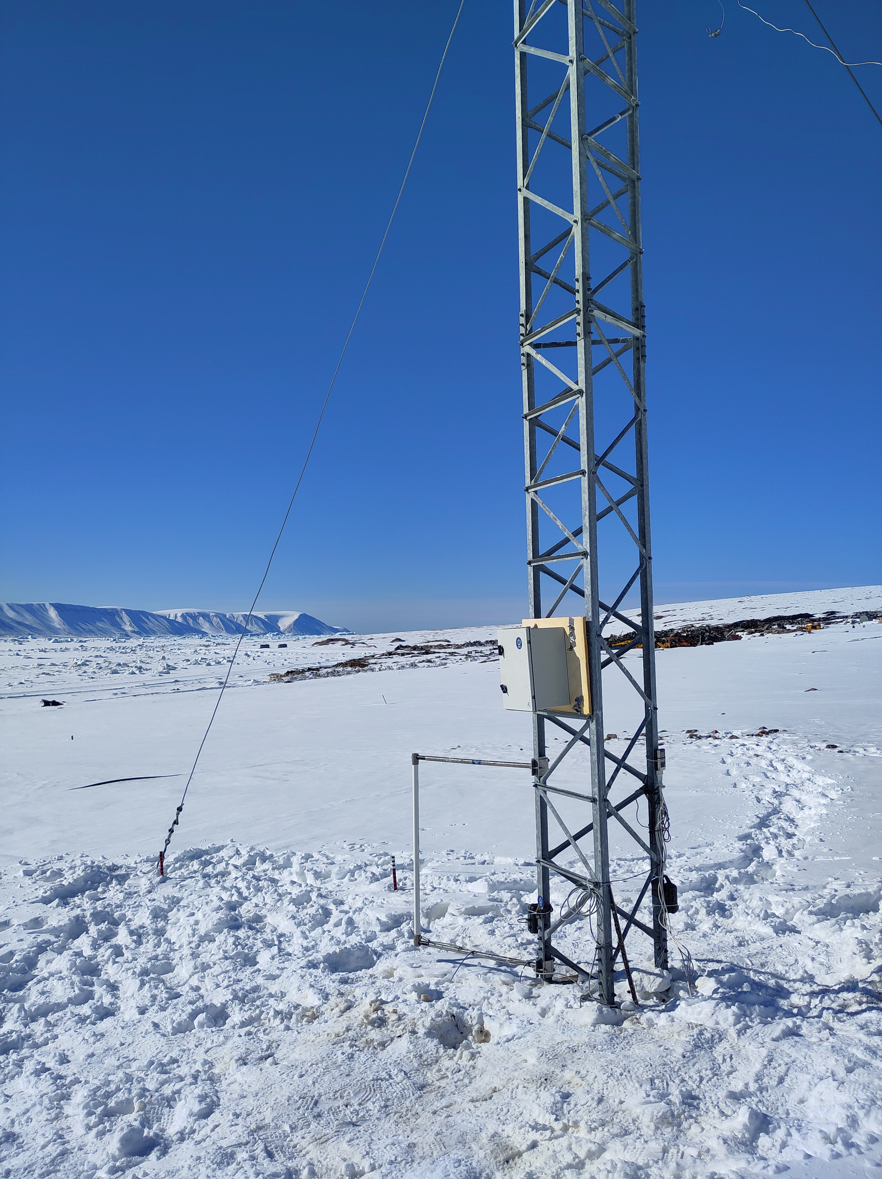
Day 4 was pretty typical of the highs and lows of fieldwork. We finished (or I should say my colleagues finished) a new mounting for the snow site logger box so hopefully the icing problem will be reduced, we (re-)installed all the instruments except for the new loggers and generally tidied up. It’s looking pretty nice now. This was a high.
Then, I struggled and failed for about 4 hours to try and get the snow drift sensors to talk to the new logger. That was frustrating low. low. However, a walk around on the fast ice in the bay to try and take a new sea ice core was some valuable breathing space – a little bit of rewiring later and the first numbers started ticking in as planned…. Hurray! That was a high!
It’s immensely satisfying solving these kind of problems. And it was the first time I’ve programmed one of these loggers – new skills are also always rewarding to learn, even if the process is frustrating. I’ve learnt a lot about SDI-12 interfaces and how the instruments actually work too. I need to remember to give myself more deep work time back in the office too. It’s much more personally rewarding and advances the science much more than endless emails and meetings.
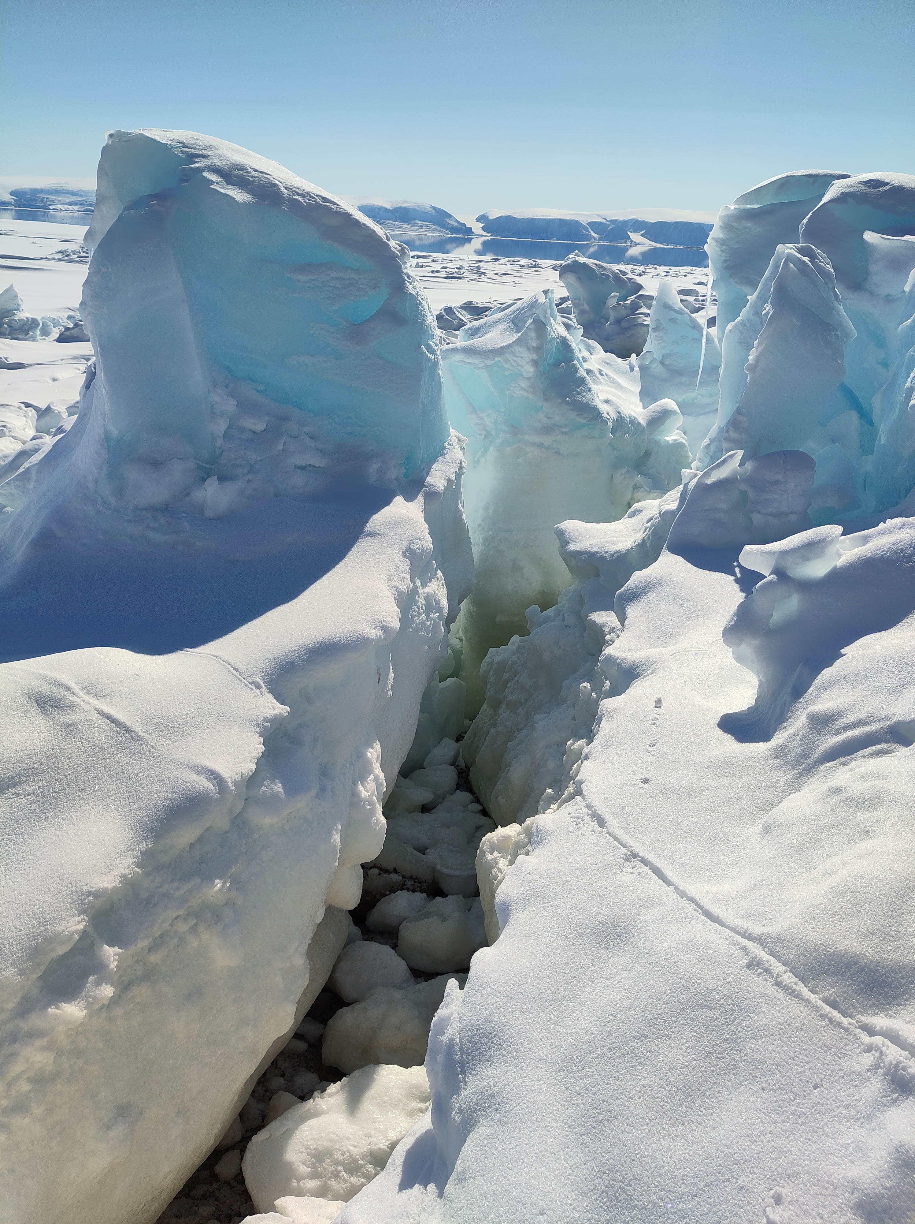
While the attempt to get an ice core was interesting, ultimately we failed due to very broken and uneven ice that made access to the part of the sea ice we wanted to get to with our kit too difficult – that was a low. I am simply counting the attempt as my evening walk, in which case maybe it counts as a high? I’ve often thought of Caspar David Friedrich’s famous Arctic painting The Sea of Ice in the coastal part of the fast ice. It’s spectacularly fractured and churned up, though FReidrich’s ice blocks are a little too angular – the real sea ice flakes are a bit more rounded.
We also did lots of preparation for day 5’s trip to the local glacier, planned a final UAV structure-from-motion mapping campaign on land and got software working to download data on permafrost from sub-surface loggers for colleagues at the University of Copenhagen – that will all however have to wait until tomorrow, our last full day in the field. Today, we have a date with a tiny local glacier.
Day 3
I’d originally assigned only one day in the fieldwork plan for the snow site work, but given we missed our prep day to go directly into the field, we have missed a few crucial steps, so we have been busy today trying to catch up, but mostly in the workshop here at the DMI geophysical facility in Qaanaaq with a couple of visits out to the snow site.
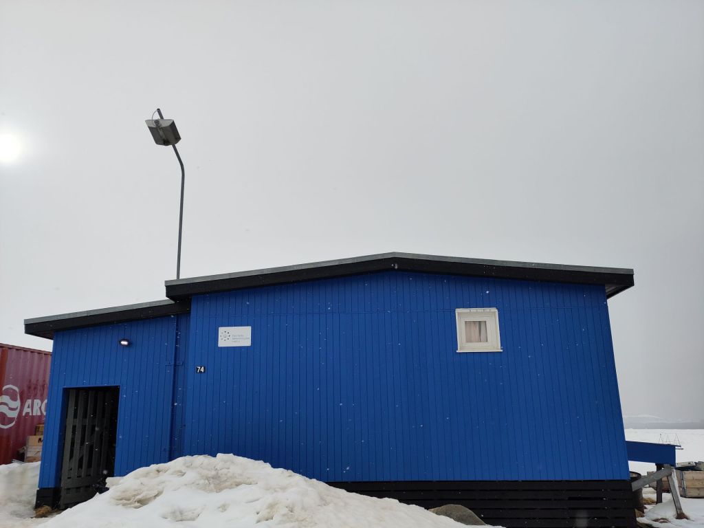
I realised I haven’t introduced the snow site.

It is a small area on the edge of the village (unfortunately near the town dump, but otherwise perfect) where we are conducting a long-term (hopefully) series of observations – we’re currently only at the end of the first year so there are a few teething troubles to sort out. We’re installing a new logger for our snow drift sensors, adding a new snow cam and downloading data from the current one. We also have a standardised set of measurements of snow properties (density, temperature, reflectivity) that we carry out whenever time and opportunity permits, that we will hopefully use to better understand how the snowpack evolves through time. The land based side is a kind of complement to a longer set of observations I have from throughout the region – all point measurements made at rather random times and locations, so the constant monitoring site will hopefully help us to understand the wider context in space and time of those point data. In fact I have a student workign on digitising that data now, so I hope to soon make available the whoel dataset for research purposes.
Snow is incredibly important in the Arctic: it forms an insulating layer over sea ice that prevents futher formation in the winter, but also helps to stop or delay surface melt in the spring and summer. On land, the insulating properties of snow also help to preserve vegetation, insects and mammals through the winter, with specific vegetation assemblages being very much determined by the local snow patterns. And that’s without even discussing the importance of snow to glaciers and ice sheets.

However, it turns out to be difficult to measure when it falls, difficult to work out how much blows around, challenging to model when it melts and when it refreezes and generally a larger than we’d hope uncertainty in weather and climate models. Much of the work developing parameterisations that describe snow properties has been done at lower latitudes too. High Arctic snow is certainly different in many respects to more southerly locations and that needs to be accounted for.
Hence the establishment of our snow programme. Which sounds rather big and impressive, but we’re hoping to set it up sufficiently smoothly this year that it will almost run itself with minimal input from us and assistance from colleagues. Let’s see, there are still some teething troubles to sort out.
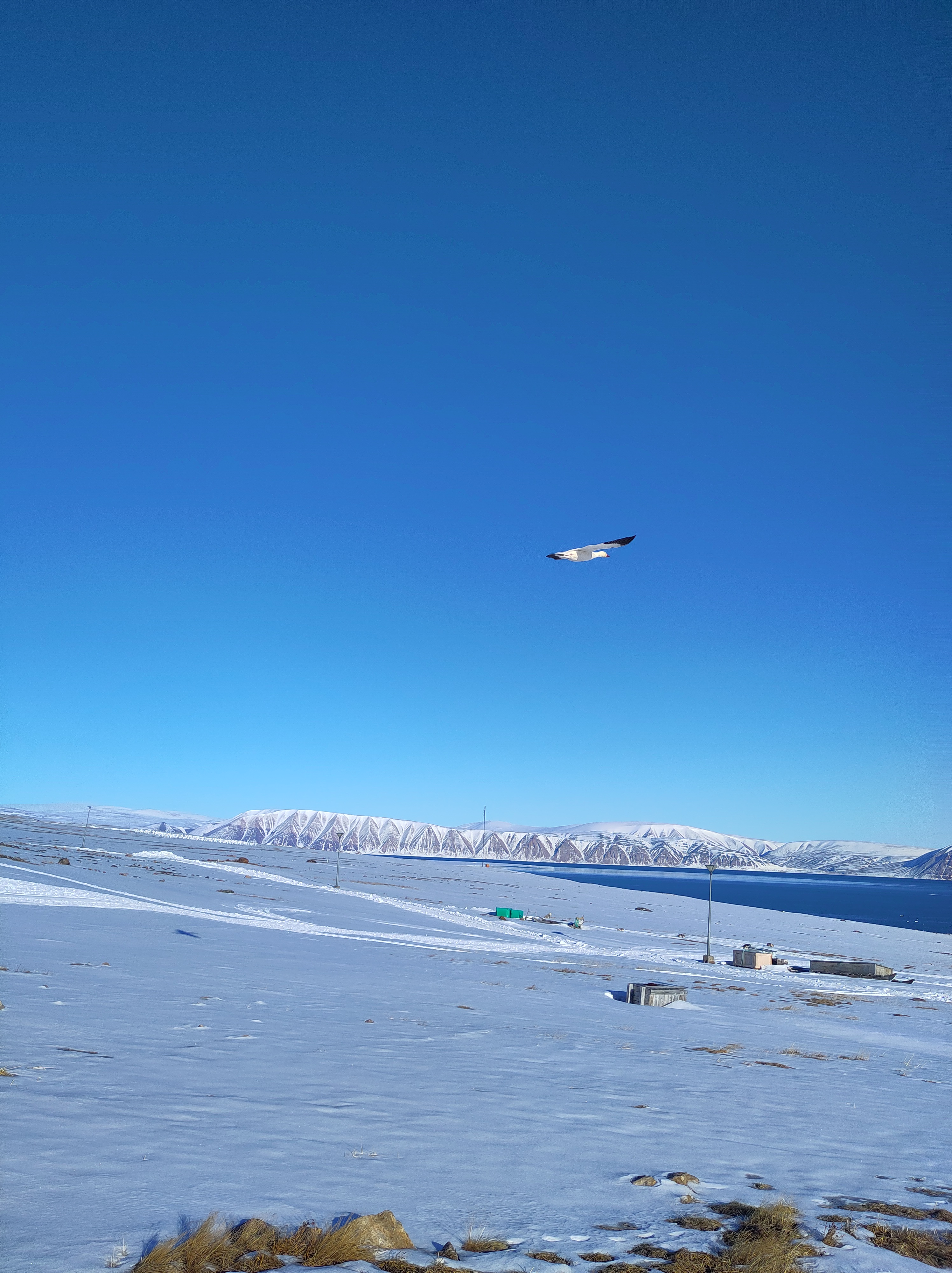
The sea ice has now cleared out of a huge part of the bay in front of Qaanaaq and the hunters have been busy taking boats out from the edge of the ice so there are clearly narwhals expected soon. Although, we’ve spent most of the last two days indoors, I keep looking outside, hoping to see some of the marine mammals that visit here. There are already masses of sea birds arriving. Yesterday managed to spot a rather handsome snow goose couple on my evening walk at 11pm.
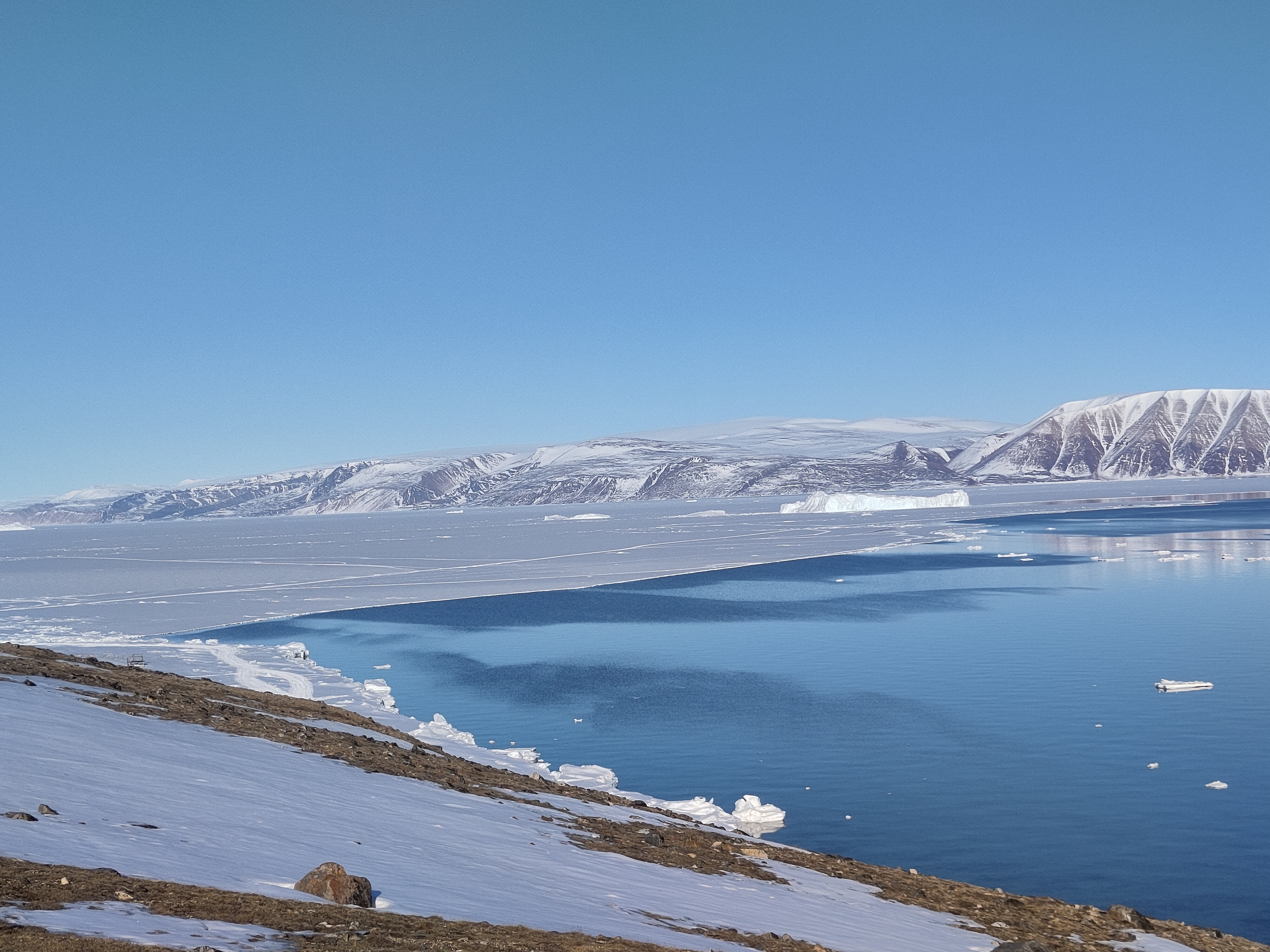
On my evening walk today I went to the very eastern edge of the town to get a look at the sea ice in the fjord – it’s quite clearly retreating rapidly now; much of the area we travelled over on Friday has gone.
Day 2
After Day 1’s rather hectic and busy time, Day 2 was assigned post-processing status. We had a slightly later than the 6am start yesterday, and put some serious effort into assessing our results from the previous day. That means downloading data, clearing up wet kit to dry it off properly, repacking stuff we don’t need further. Then there is the computer work, doing some initial processing, backing up files, writing field notes and doing some measurements (of salinity) on the sea ice cores we collected.

We also made time to visit our snow site to download data from the instruments there. Unfortunately, it was clear that we need to somewhat reorganise the site, the logger box was completely snowed in, and I was a bit sceptical there would be any data at all. So we collected in some of the instruments for testing and further data downloads in the workshop instead of trying it out in the field. In fact, fieldwork means a lot of tidying up and computer work! I used the opportunity to reorganise and standardise the way we archive all our data, including the UAV images as well as the meteorology instruments, which will also hopefully mean we have an easier time to find and use it in the future.
It wasn’t all laptop work though, we did a few snow pits and some further testing of the Infrasnow system we have borrowed. I’m actually quite impressed with it – very straightforward to use and very consistent data produced.
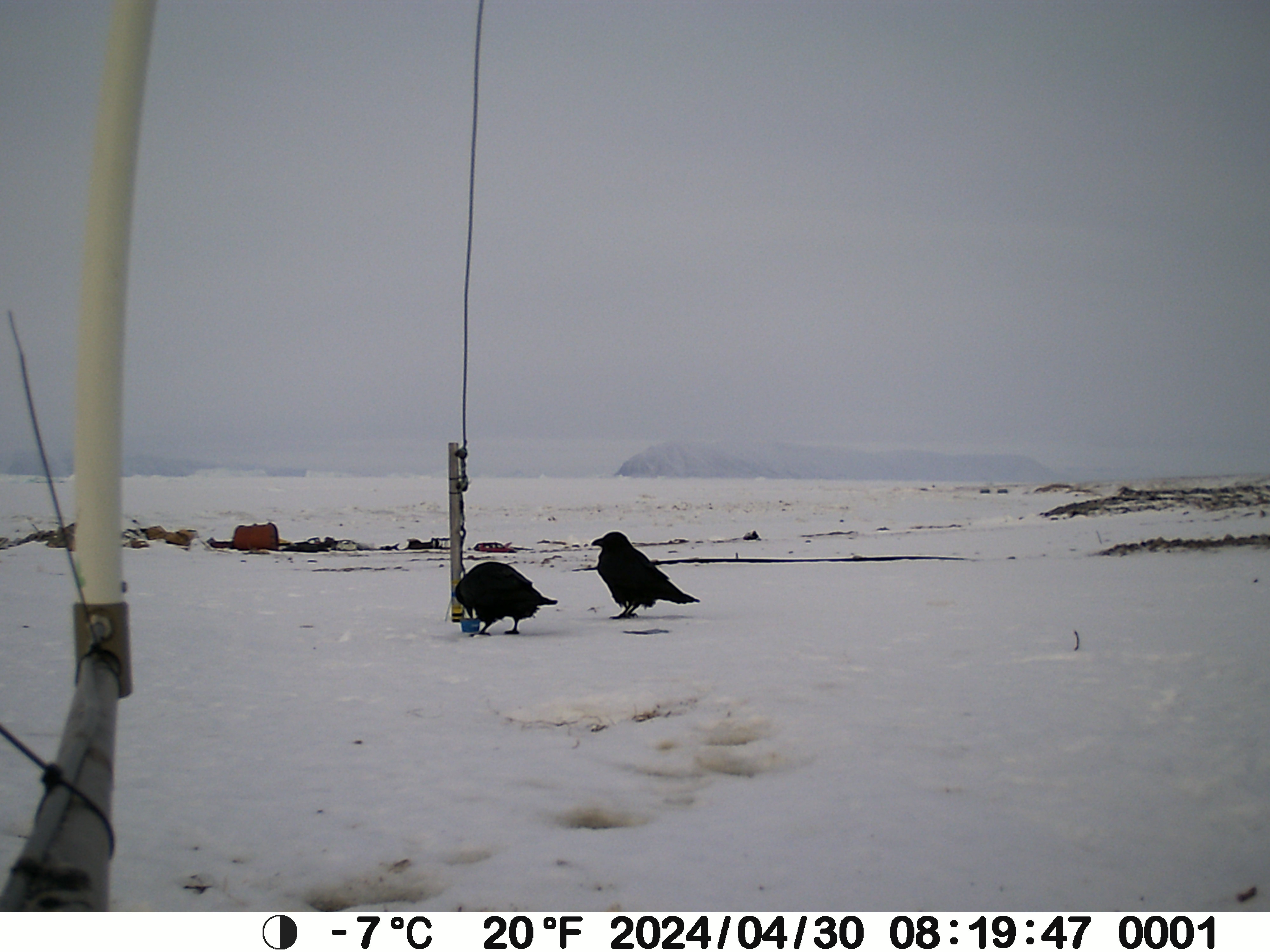
It’s also always fun to check our snowcam – this takes a photo of a stake every 3 hours to monitor the depth of the snow pack, and quite often we get beautiful views and some cheeky ravens hopping past too – I live in hope for an Arctic fox, or even a bear.
On the subject of bears, I had heard there were rumours of one near the snow site, but sure enough there were the footprints – rather small and filled in with snow but quite distinctive and heading up towards the ice cap. We shall be extra careful when we go up on to the glacier later this week.
Day 1
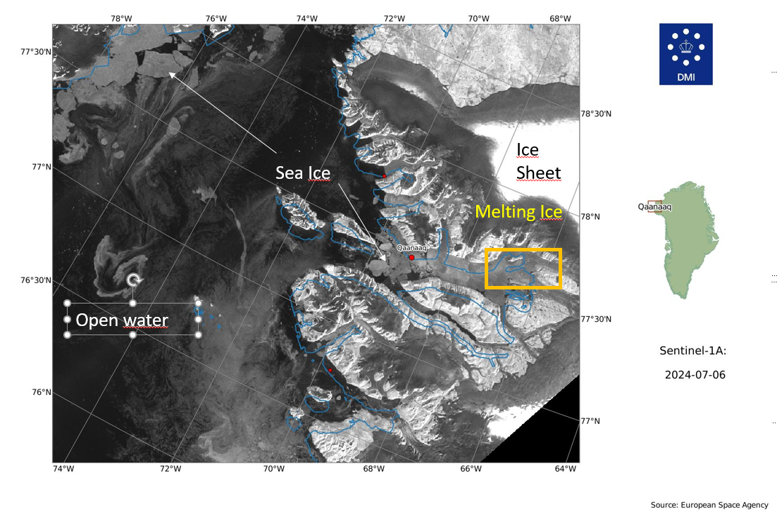
We had originally planned terrestrial, glacier and sea ice work, primarily focused on snow processes. The sea ice part though was altered and expanded when the rapid break up in April and again this month was observed. Normally, we’d have a preparation day between arrival and going into the field, but the threat of winds and high temperatures meant we decided not to risk it and we went out straight away on the first full day. Our instincts to just go yesterday turned out to be correct, we had perfect weather and with the help of Qillaq, one of the local hunters we still made it out on to the sea ice. So all is not lost. I woke up this morning to see a wide blue sea just off the last pieces of fast ice on Qaanaaq, so I’m very happy with that decision. Sentinel-2 captured this yesterday while we were out in fact.

It probably looks more dangerous than it is. We were working on the stable fast ice to the east of the big flake, that stretches right into the fjord. The local topography make it very stable and our measurements yesterday confirmed it’s pretty typical for the time of year in thickness, though there was a surprising amount of snow on top, which can actually help to protect the ice from melt at this time of year.
Getting around the coast was surprisingly straightforward, the fast ice has a very stable platform, though some large churned up part of the ice with cracks made for some slightly bumpy manoeuvres to get on and off the stable parts.

The dogs were I think happy when it was over. But in fact it was much more straightforward than I’d feared. The large crack we noticed earlier in the week that opened into a wide lead further extended while we were out, see below, and I woke up this morning to a wide open lagoon. It’s an extraordinarily beautiful place to work and I feel so privileged, especially on days like today when the weather is also being extra nice.

Work wise it was a successful day, we managed 2 stations, where we did very extensive work. I’d have liked a third but the deep snow made it very heavy and slow going to travel on and in spite of the early start we basically ran out of time and had to return home.

We flew the UAV for surface properties, did a lot of snow pits and snow surface properties work, drilled some ice cores (which I will be working on this morning) and even got our loaned EM31 working to do automated ice thickness mapping. We will hopefully start to look at the data later on today to make sure it makes sense before we leave on Thursday.

The reduction in ice means we can actually concentrate on the terrestrial part of the work plan for the rest of the week. And there’s a lot to do!
Last year I set up a semi-permanent snow site to monitor conditions on land through the year. It is going to get a bit of an upgrade this week with some new instruments and of course we need to get the rest of the data downloaded and processed from here too.
Onwards.