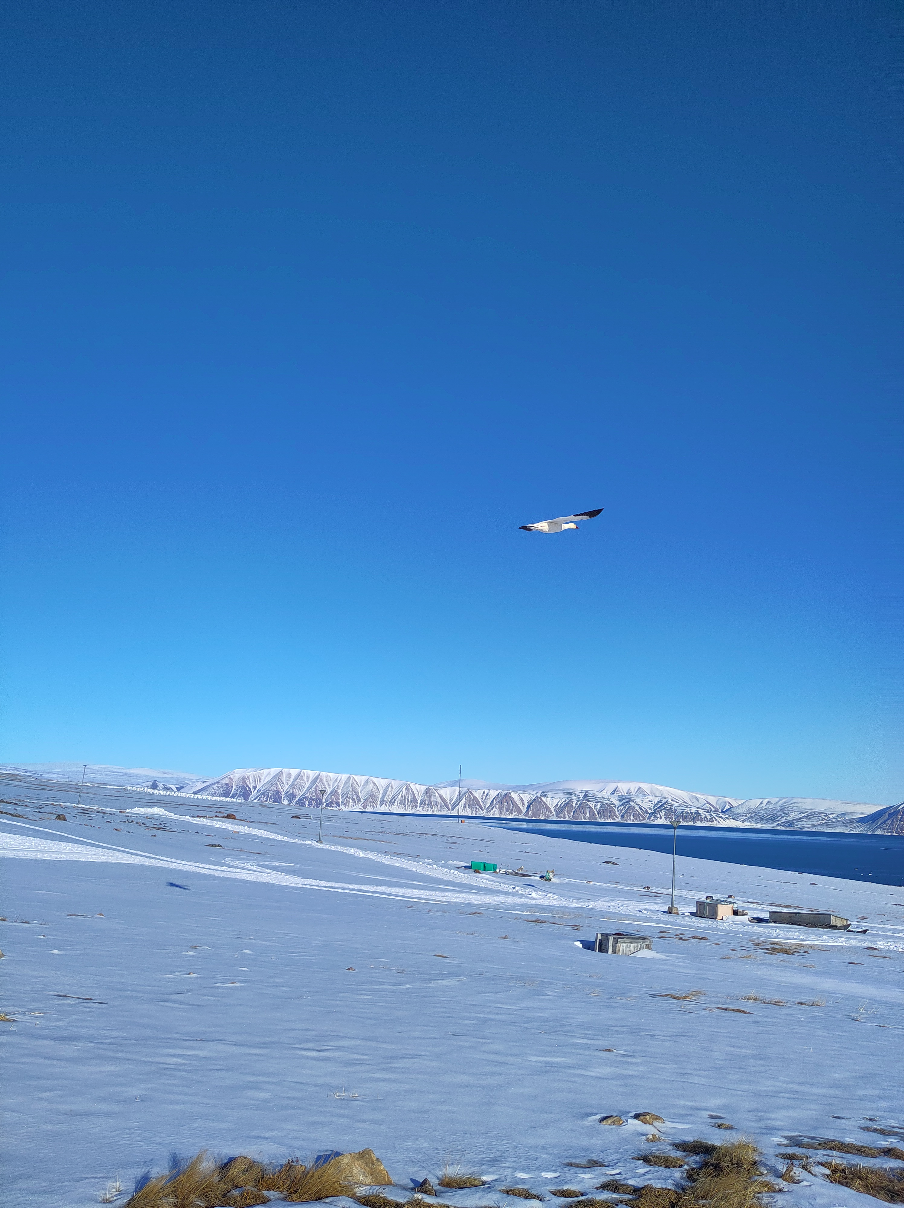
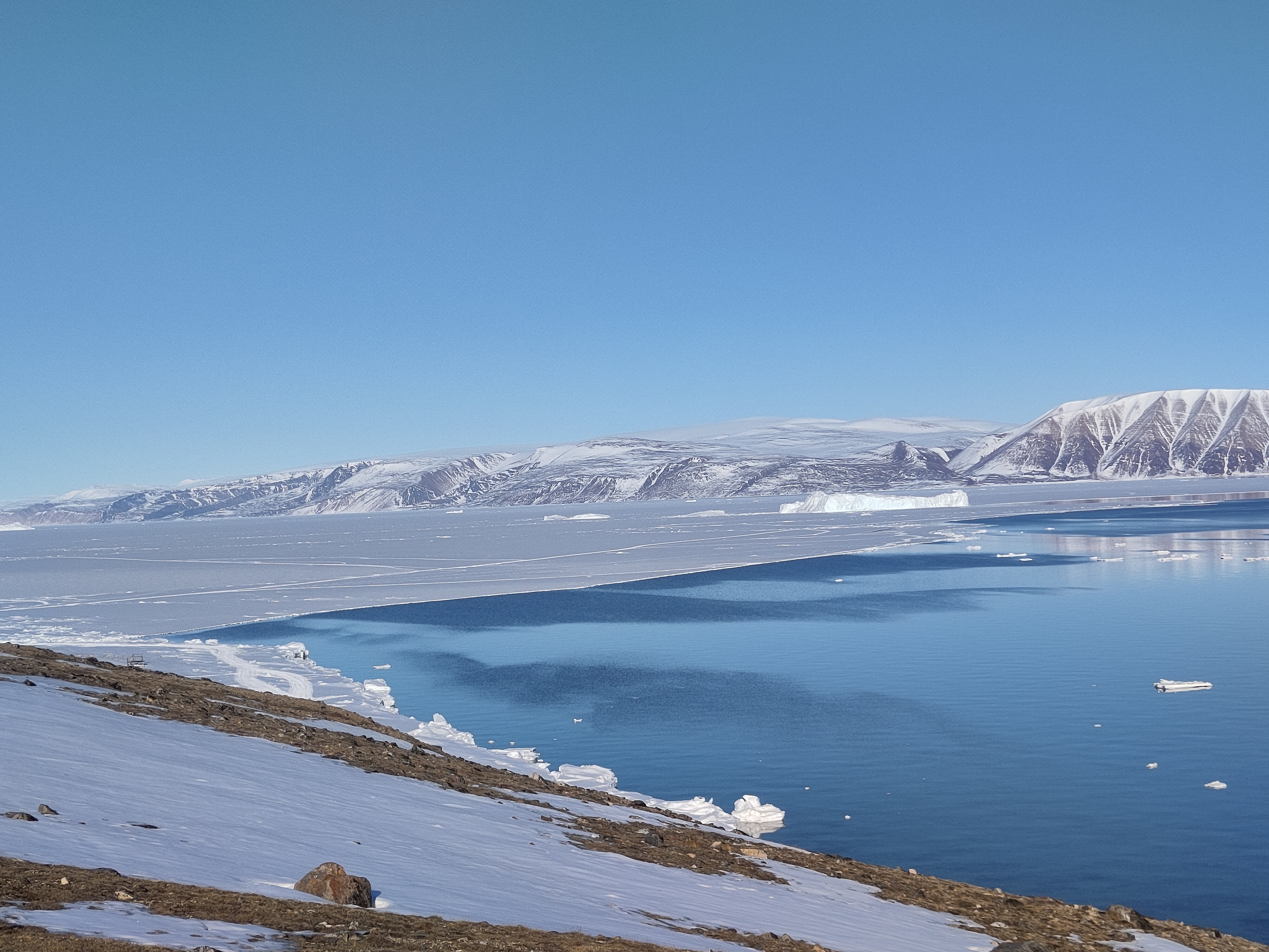
I’m in Antarctica and yet I have been getting contact from journalists because Greenland is all over the press at the moment for all the wrong reasons. It’s reasonable I think to worry about what the various deranged threats towards Greenland will mean for us all also outside of Greenland. But I also think about (and yes, worry) about the friends I’ve made in Greenland over the years. Let’s hope common sense prevails and we can step back from the brink, and concentrate on the really long term problems that we are still rapidly storing up for ourselves.
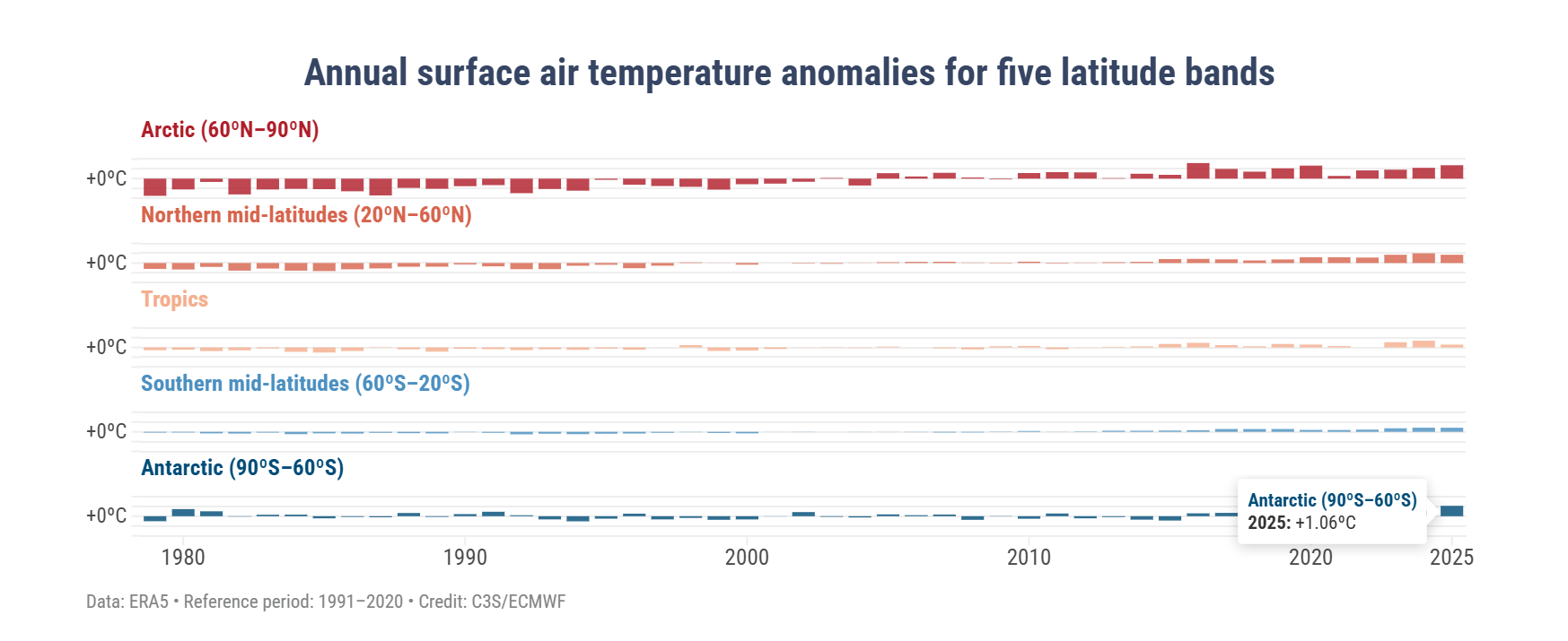
Greenland is also on my mind, not just because of geopolitics, but also because the Copernicus Climate service has just put out their annual global climate highlights* for 2025 report with some disturbing results from Antarctica.
A few months ago we had a paper published called the Greenlandification of Antarctica, in which we argue that the changes in the Antarctic cryosphere increasingly resemble those we have previously observed in Greenland and the Arctic. To see the future of Antarctica, look at Greenland.
It’s been a busy time preparing for fieldwork and I didn’t manage to write anything here about it at the time, but this few eye-opening figure rather supports some of our arguments.
In this graphic, the 2025 temperature over the Antarctic region was 1.06°C higher than the average between 1991 and 2020 (a temperature anomaly). This is actually higher than any other region except the Arctic, where the temperature anomaly was reported to be 1.37°C above the 30 year average (bear in mind also that between 1991 and 2020, the temperature was also much increasing, so we’re not comparing with a pre-industrial climate here). Polar amplification was predicted long ago and as those first experiments found, it also is seen more in the Arctic than the Antarctic – but these results are a first hint of the amplification that is perhaps appearing now and may come to stay in the Antarctic.
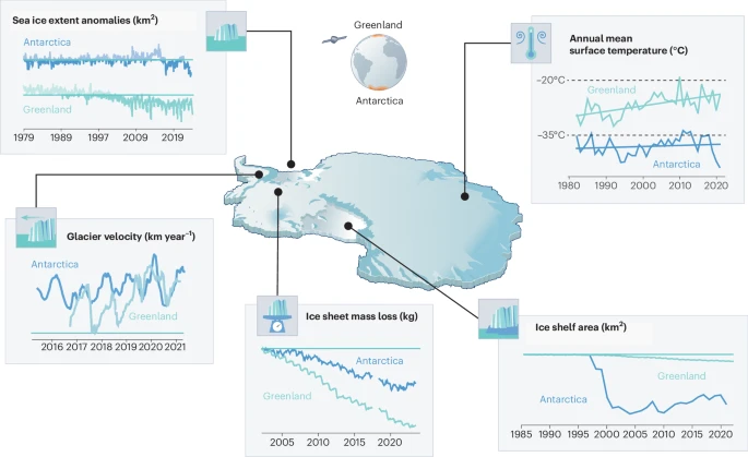
In our paper we show the figure below (many thanks to illustrator Jagoba Malumbres-Olarta for the fine work), which shows five different cryosphere properties that are changing: 1) shrinking sea ice, 2) glacier velocities that show a seasonal cycle (mostly detected on the peninsula so far, though there are indications that Totten glacier for example has some kind of seasonal cycle, possibly modulated by sea ice), 3) total ice sheet mass loss, 4) ice shelf area and 5) annual mean surface temperature. In virtually all, the changes look very similar between Greenland and Antarctica, but with the crucial difference that the speed of changes is so far faster and more advanced in Greenland.
From Mottram et al., 2025: The Greenlandification of Antarctica. Original caption: a, Commonalities include decline in sea ice extent from 1980 to 20232, with notable step-like changes in both poles. b, Seasonal glacier velocities are shown for two representative marine terminating glaciers, Kangilernata Sermia in Greenland13 and Hotine Glacier on the AP9, both now displaying similar seasonal dynamics. c, Both ice sheets show an accelerating total mass loss measured by GRACE satellites8. d, Multi-sensor records of ice shelf area loss in Antarctica11 show a steeper decline than Greenland7 as Arctic ice shelves were largely lost in the pre-satellite era. e, Satellite records of annual mean ice sheet surface (skin) temperature for 1982 to 2021 from radiation data in the CLARA-A2.1 record processed by OSISAF2 over both ice sheets. Earth observation data allows us to generalize over the vast size and spatially varying trends of the ice sheets, where there is generally poor coverage of in situ data. Individual weather stations indicate warming trends in air temperatures over both ice sheets of ~0.61 °C per decade at the South Pole and ~1.7 °C per decade at Greenland coastal stations. Illustration by Jagoba Malumbres-Olarte
The latter surface temperature plot is not the same as the Copernicus 2m air temperature which is based on the ERA5 reanalysis (so a blending of computer model with observations from satellites, weather stations, balloons, ships, planes etc). In our paper we wanted to focus on the contribution that satellite data has brought as we simply have so few direct in situ observations, so we used skin or surface temperature which is measured from satellites. It’s a somewhat theoretical construct, imagine a very thin surface (hence skin) layer, where incoming and outgoing energy are summed up to give a temperature. This is calculated over both ice sheets and sea surface by our colleagues in the satellite group at DMI and this is the dataset we used here. Their results which stretch back to the 1980s show a slow upward trend in Antarctica and a steeper change in Greenland, the record stopped in 2021 in our paper but it actually shows an upward increase since and that’s also borne out by the Copernicus results. In climate and weather models we in fact first calculate the skin temperature and then back interpolate to 2m temperature, so the two are very closely related.
To check that the satellite skin temperature record was accurate, I also looked at some of the longer in situ records, the South pole station for example has a long record and shows a small increasing trend over the last 30 years or so (which also may be attributable to natural causes, it is hard to pick out the global warming trend). Analysis of the record also shows that it is largely due to decreasing cold extremes rather than necessarily higher warm extremes. Again, a pattern we also observe in the Arctic.
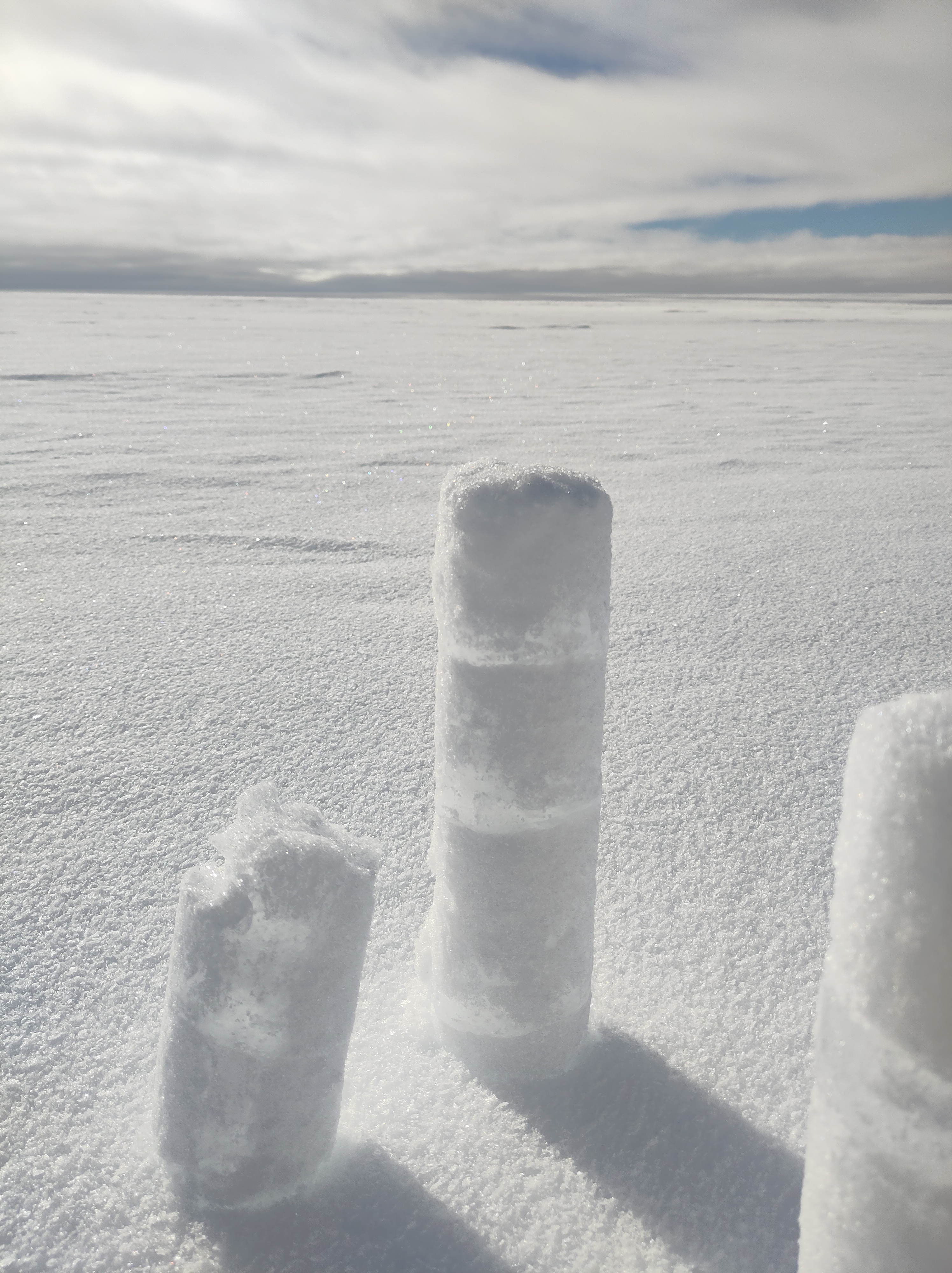
Shallow snow cores drilled near Wasa, the clear layers are refrozen surface melt that has percolated into the snow below the surface. I was genuinely not expecting to see these, and it’s not always captured in the satellite record either, so we clearly have work to do to explain some of these findings.
The analogy is not exact. As a continent, Antarctica is much further south than Greenland is to the north and it is much more insulated from warming by the circumpolar ocean than the Greenland ice sheet, sticking out in the middle of the Atlantic is. In a very real sense then, geography is destiny. Surface melt, which is also not nearly as common here in Antarctica mostly refreezes in the snowpack, whereas in the lower parts of Greenland it generally runs off and contributes directly to sea level rise. That has not yet become a major process in Antarctica, it’s still colder here and there is less surface melt for now, although from our own observations in the field, much more than I’d expected. Surface melt is definitely something we need to keep an eye on and some of our observations show how tricky that is, especially given disagreements between satellite sensors on this point .
But these are all details, the point is that Antarctica is also part of the global climate system and the same processes we’ve been observing for more than three decades in Greenland are now also starting to become apparent here too.
In one other respect Antarctica is becoming more similar to Greenland – it is becoming more contested. The Treaty that has governed Antarctica is vulnerable and subject to the same weakening of the global order that is now playing out in the North.
Let’s hope that geopolitics can settle down soon so that we can start to tackle the more serious and longer term crises coming down the line.
*I’m not sure “highlights” is quite the right word either – maybe “lowlights” would be better, but then it also starts to sound like a report on hairstyles…
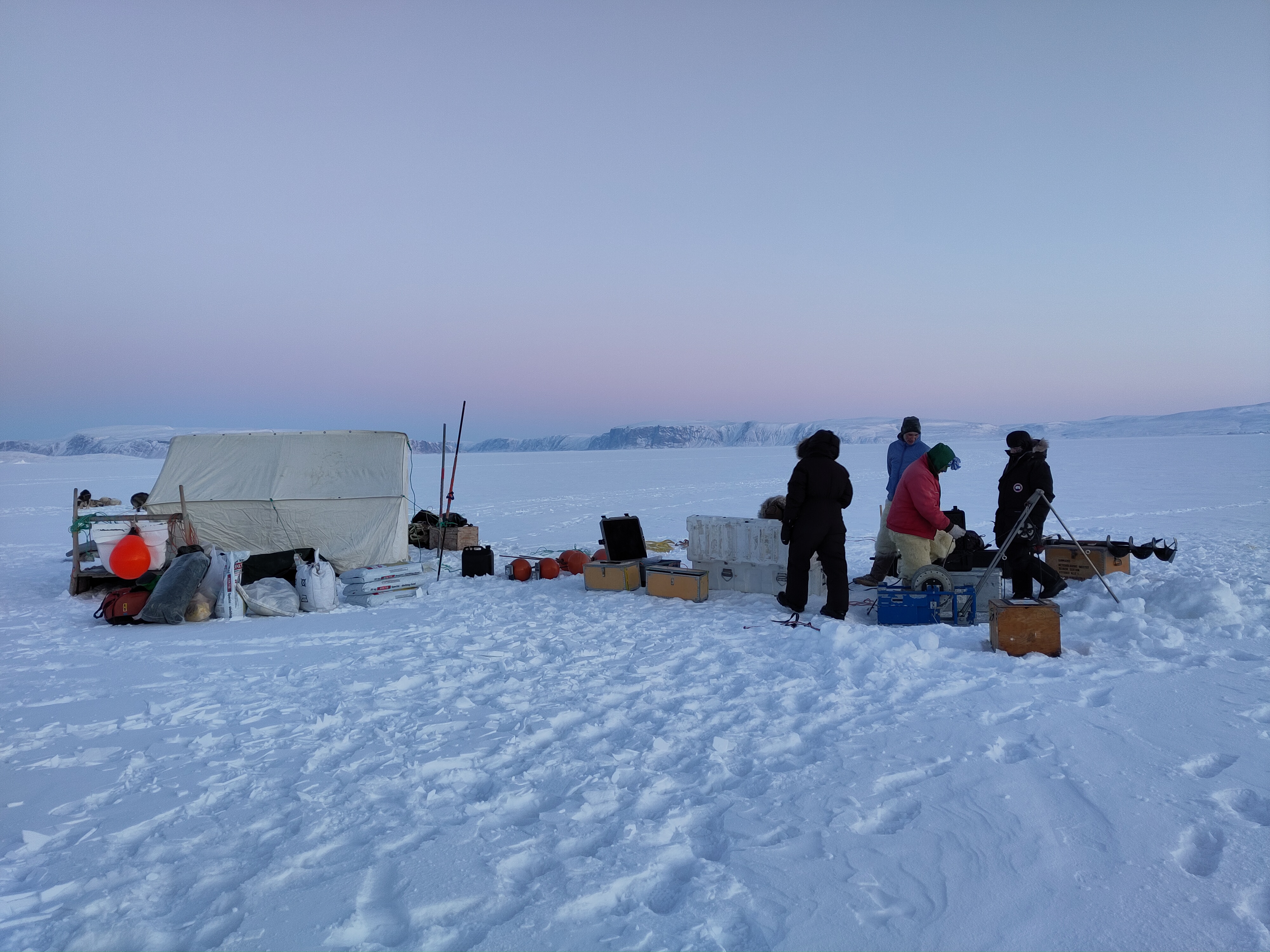
I very rarely have time to write a proper field diary, our time in the field is usually extremely hectic and filled with 12-18 hour working days that blend seamlessly together. I suspect this week is also going to be busy, but Nature has offered an olive branch in the shape of an early break-up of the sea ice, so I’m taking a moment to write a few things down. Updates will be posted at the top so scroll down to read the first day.
And finally…
I’m writing this on the metro home, I’ll spare you the flight delays, the packing up dramas, the last minute, “just one more snow pit”…
Melville Bugt from the air
It was a good tour. Enormous amount of work done, perhaps more importantly, it has also been foundational work, on both data and field site management, it will be much easier for colleagues to help us maintain this and to build up a long term data set of all the observations (and more that I haven’t written about here) in future. That should reduce costs and field time in the future but also give others the opportunity to visit and do their own research up here.
The traditional hunters gloves turn out to be by far the best thing to work in when programming outside. You can put your hands in and out very fast and they are super warm.
I think streamlining the storage of data is extremely important. There is far too much data in the world on hard drives and in field notebooks, doing no good to anyone. This system will be much easier for other colleagues to use what we have collected and we will be able to publish them outside of DMI soon too. I remain committed to FAIR publishing, but I often feel the barriers are practical rather than psychological.
I’ve also introduced my new(ish) colleague Abraham to the Arctic. Given he grew up in a place without snow it has been a delight to watch him discover the processes and problems that I’ve been working on the last 20 years and that we’ve been discussing together the last 18 months. I believe it’s extremely important for climate modellers to understand and see the system they’re trying to model. This trip has definitely confirmed me in that. This was not just a field campaign but also a pedagogical field trip in some ways too. We have also had the opportunity to brainstorm a lot of new research ideas along the way, there is rarely such time in the office, so plenty more to work on in coming years..
The DMI geophysical facility, newly painted!
As ever massive thanks to many colleagues, especially Aksel our DMI station manager without whom this work would be close to impossible given he is both interpreter and collaborator on the practical observations; Qillaq Danielsen for taking us out on to the sea ice with his sled. Steffen for running an extremely valuable long-term programme, Andrea for helpful and practical discussions and of course Abraham for making it a very good week. Glad we got to do this.
I should also say a large thankyou to my husband for keeping the home front running smoothly along whilst I am travelling. None of this would work otherwise.
Tak for denne gang Qaanaaq!
Day 6: Last day
It’s amazing how fast the tine goes, our last full day in the field (we’d originally planned for 9 days, but that was partly because last year we planned a week and it got cut to 3 days due to flight weather problems, I learned and left a safety margin this year). Nonetheless, a busy day. As we’re really interested in lots of different processes that combine in what we call the Arctic Earth System our focus for today was twofold, looking at the atmosphere and the subsurface, both of which are partly other scientists projects, but giving data we really want to use with our climate model, both for evaluation and development.
Aksel and Abraham giving the site a few last tweaks
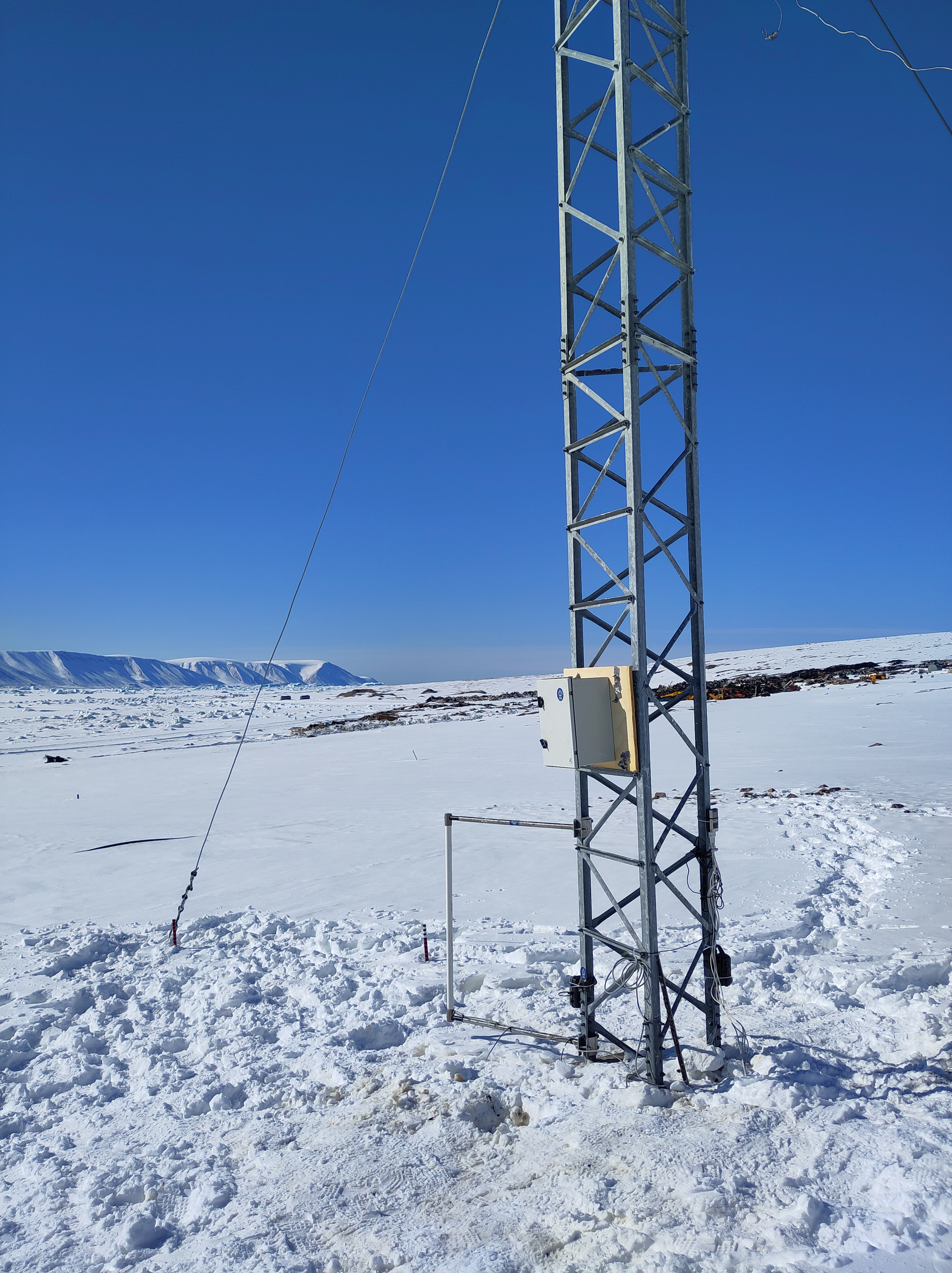
The main aim was to finalise the snow site ready for observations over the next year. We finally reinstalled the remaining FC4 and new logger, this has been ticking over and being tested in our station kitchen for the last couple of days. I’m rather pleased with myself in managing to get these 2 talking to each other, I was envisaging a bigger struggle, but the Campbell Scientific software is very easy to use with good user guides.
The installation was the last element for the snow site and after Aksel and Abraham’s sterling work in building our new logger station, it was trivially easy.
Et voilá! We have a fully functional snow site…
The experience with the new Campbell system proved invaluable in the next task, downloading a whole bunch of data from colleagues’ weather stations for shipping back to Denmark. Normally, we would have been a bigger crew to handle work on the sea ice as well as at the station, but as the sea ice broke up so early (see Day 1), our local hunter friends had taken them down and brought them in to Qaanaaq for us. They needed a bit of repacking, data downloads and checks and we set up a skin temperature calibration station for the satellite group, which I think will also be quite interesting for us in polar regional climate modelling to use. This we left overnight for longest possible calibration.
As we have many collaborations we also spent an hour trying to collect some data from the subsurface permafrost sensors installed by our colleagues at the University of Copenhagen. Unfortunately, it appears they need rather more maintenance than we can provide, so that will need a full team. I am extremely keen to see the data though, ten years + of permafrost and temperature measurements is a seldom dataset and will be super interesting to use in the further development of our surface scheme. Qaanaaq is somewhat vulnerable to permafrost disturbance as it is built on sediments, so monitoring this in a warming climate is pretty important.
A long day, but made even longer by the excitement of narwhals in the bay! We headed out to the ice edge at 11pm, (the polar day plays havoc with your body clock), where quite a few hunters had gathered and were busy slicing up a freshly caught narwhal, eagerly filmed by at least one of the several film crews and photographers there appear to be in the town right now. We have noticed increasing numbers of film crews visiting this part of the world. It can be surprisingly busy.
Greenland does have a strictly regulated quota on narwhals, it’s an important part of the culture, but it is a bit brutal to watch if you’re not used to seeing animals sliced up. Personally, I think everyone should see where the meat they eat comes from. It would make us all more honest about agriculture. But I digress, I was actually more excited to see live ones out in the bay. We’re immensely fortunate to see them, this is only the 2nd time in 5 years I have seen live narwhal here, and it’s only really because the ice has shrunk so early allowing them in. I have immense respect for the hunters who go out in flimsy lightweight kayaks to harpoon them. That must take some courage.
It’s such a peaceful scene, hard to imagine the life and death struggle implied here.
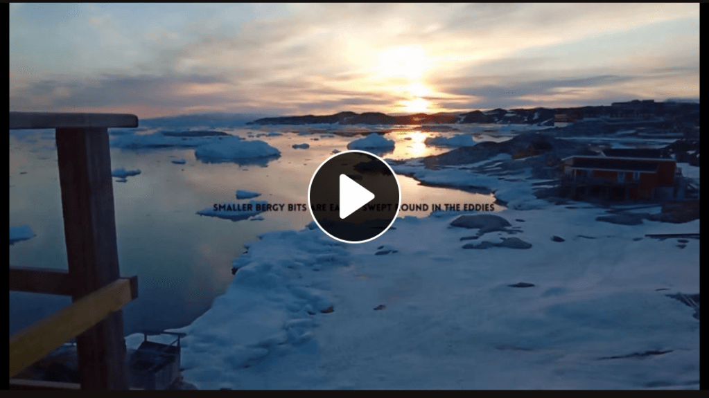
UPDATE: And as an aside, our ace colleagues and collaborators at the Greenland Institute of Natural Resources have a wonderful series of videos exploring all kinds of research in Greenland, including this brilliant one featuring Malene Simon Hegelund and my DMI colleague Steffen Olsen, together with Qillaq Danielsen who we were also out with this year, which really gives a flavour of fieldwork in Qaanaaq and just how important our collaborations with the local community and Greenlandic scientists are.
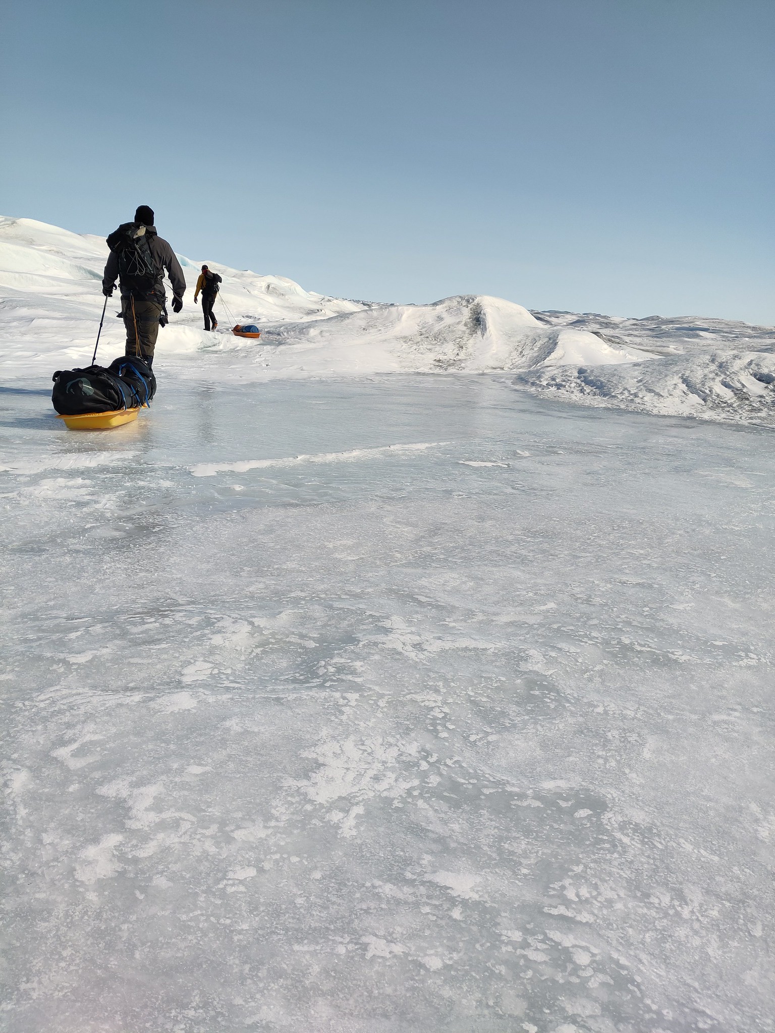
Day 5: Glacier Day!
As an unrepentant glaciologist, I always look forward to glacier day, when we get up onto the land ice. In this case it’s only a tiny outlet glacier from a rather small local ice cap (well I say small, in the Alps it’d be considered quite large, but by Greenland standards it’s small but well studied). It’s easily accessible and the point about today was to take surface snow measurements and density profiles, so accessible is good.
The deep soft snow that has been a bit of a bane everywhere this year was also a problem. It was very heavy going, there isn’t really a path, just very loose rocks in a (at this time of year dry) riverbed, which is bad enough in summer but when covered in 30cm of snow was quite heavy going. Nonetheless we made a decent pace and got quite high up. By the time we came down again, the outwash river was starting to show signs of life again. It was a cold day, between -3 and -5C but the blazing sunshine alone is enough to start to generate melt and we saw plenty of signs of radiation driven melt going on under the surface snow crust, especially where there were dust layers to accelerate the process.
The snow pits proved indeed how cold the snow has been, typically around -10C at the bottom of the pits, but in one we also found signs of refrozen melt water, perhaps from the brief March warm period?
Ice layers in the snow, surprisingly difficult to photograph, you’re going to have to trust us on this one!
We did a transect down with our borrowed infrasnow, made several density profiles and had quite an efficient time. The idea is to repeat this transect at different times of the year so we can see how the snow properties change. In particular, I’m interested in surface albedo (how much incoming light is reflected by a surface). The reflectivity of the snow and ice surface is extremely important for the energy budget, which in turn controls how fast the snow (and ice) melt as well as being important for satellite data retrievals of surface temperature.
The Infrasnow is a very neat device that measures density and specific surface area. It’s not quite the same thing as albedo but it will help us to develop our albedo scheme in the model as it is based on grain size. Unfortunately it does not work on glacier ice, which is some places we also saw peeking out the top where wind has scoured the surface snow away. The movement of snow by wind is the subject of our final full day in the field.
We continued the observations off the glacier all the way to the road so we have a nice base transect that can be repeated to assess how conditions change through the year.
Although we only hiked 10km, it was quite tough, so next year we’ll bring snow shoes…
Tomorrow is our final full day. Lots more to do.
Day 4
Day 4 was pretty typical of the highs and lows of fieldwork. We finished (or I should say my colleagues finished) a new mounting for the snow site logger box so hopefully the icing problem will be reduced, we (re-)installed all the instruments except for the new loggers and generally tidied up. It’s looking pretty nice now. This was a high.
Part way through the reinstallation at the snow site
Then, I struggled and failed for about 4 hours to try and get the snow drift sensors to talk to the new logger. That was frustrating low. low. However, a walk around on the fast ice in the bay to try and take a new sea ice core was some valuable breathing space – a little bit of rewiring later and the first numbers started ticking in as planned…. Hurray! That was a high!
It’s immensely satisfying solving these kind of problems. And it was the first time I’ve programmed one of these loggers – new skills are also always rewarding to learn, even if the process is frustrating. I’ve learnt a lot about SDI-12 interfaces and how the instruments actually work too. I need to remember to give myself more deep work time back in the office too. It’s much more personally rewarding and advances the science much more than endless emails and meetings.
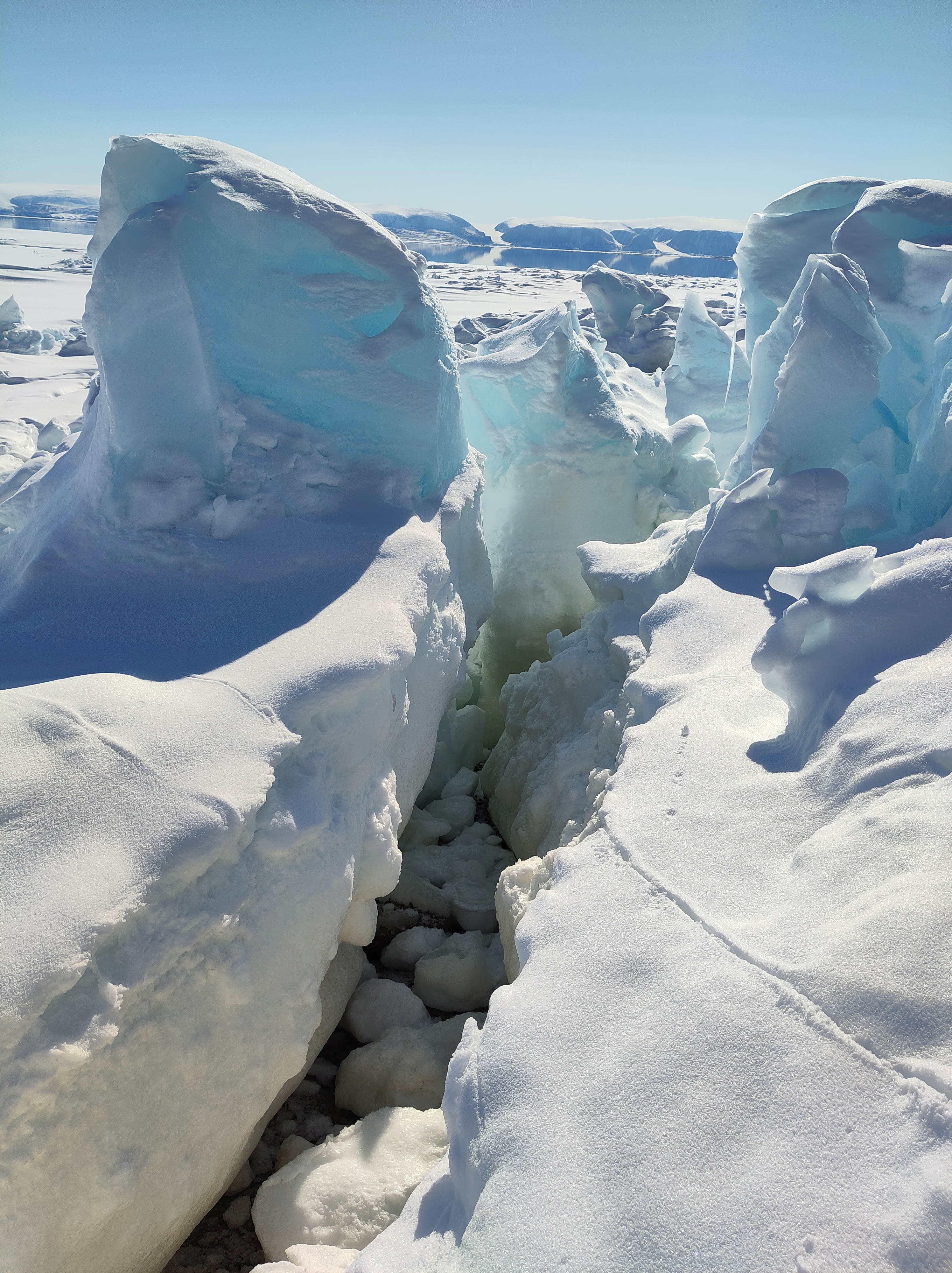
While the attempt to get an ice core was interesting, ultimately we failed due to very broken and uneven ice that made access to the part of the sea ice we wanted to get to with our kit too difficult – that was a low. I am simply counting the attempt as my evening walk, in which case maybe it counts as a high? I’ve often thought of Caspar David Friedrich’s famous Arctic painting The Sea of Ice in the coastal part of the fast ice. It’s spectacularly fractured and churned up, though FReidrich’s ice blocks are a little too angular – the real sea ice flakes are a bit more rounded.
Where the fast ice meets the land…
We also did lots of preparation for day 5’s trip to the local glacier, planned a final UAV structure-from-motion mapping campaign on land and got software working to download data on permafrost from sub-surface loggers for colleagues at the University of Copenhagen – that will all however have to wait until tomorrow, our last full day in the field. Today, we have a date with a tiny local glacier.
Day 3
I’d originally assigned only one day in the fieldwork plan for the snow site work, but given we missed our prep day to go directly into the field, we have missed a few crucial steps, so we have been busy today trying to catch up, but mostly in the workshop here at the DMI geophysical facility in Qaanaaq with a couple of visits out to the snow site.
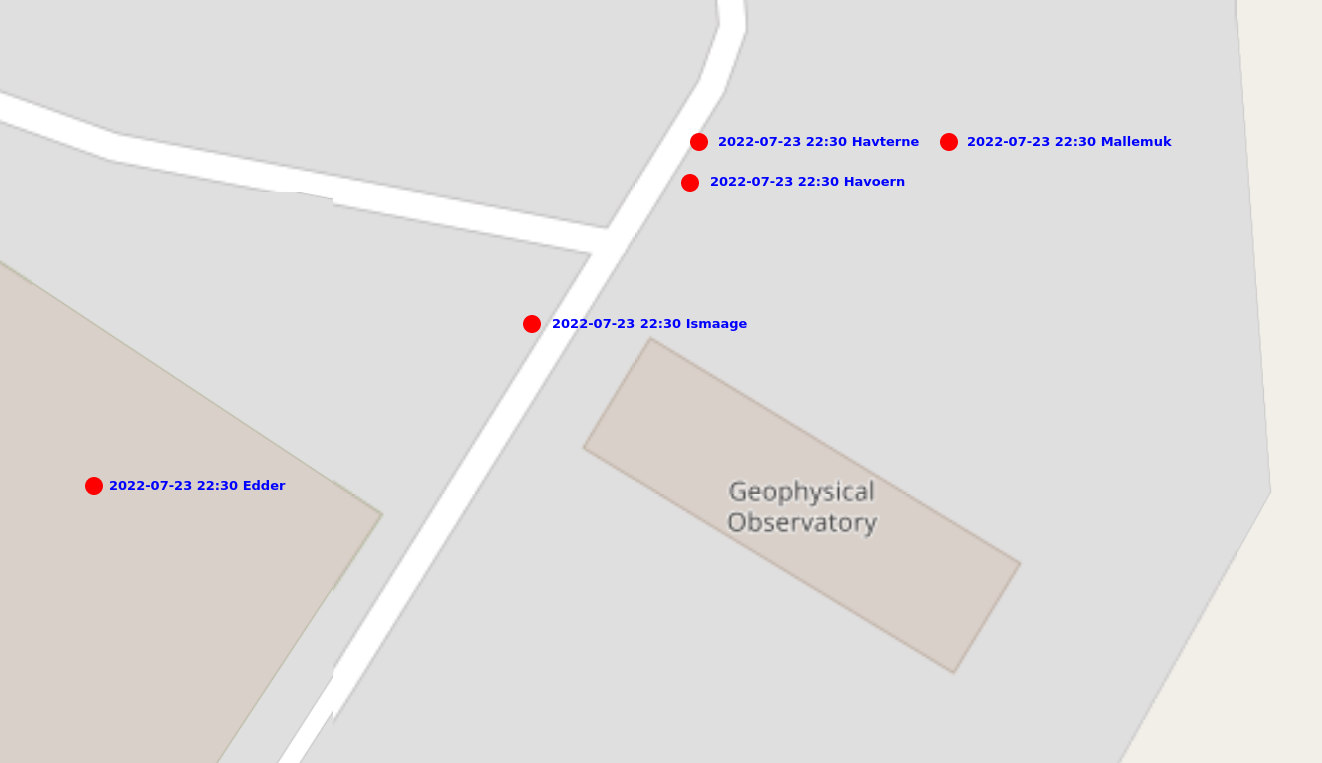
I realised I haven’t introduced the snow site.
View over towards the south west from the old ionospheric research station on the edge of Qaanaaq. Our snow site in the foreground. It has a great view, if you ignore the town dump at the coast!
It is a small area on the edge of the village (unfortunately near the town dump, but otherwise perfect) where we are conducting a long-term (hopefully) series of observations – we’re currently only at the end of the first year so there are a few teething troubles to sort out. We’re installing a new logger for our snow drift sensors, adding a new snow cam and downloading data from the current one. We also have a standardised set of measurements of snow properties (density, temperature, reflectivity) that we carry out whenever time and opportunity permits, that we will hopefully use to better understand how the snowpack evolves through time. The land based side is a kind of complement to a longer set of observations I have from throughout the region – all point measurements made at rather random times and locations, so the constant monitoring site will hopefully help us to understand the wider context in space and time of those point data. In fact I have a student workign on digitising that data now, so I hope to soon make available the whoel dataset for research purposes.
Snow is incredibly important in the Arctic: it forms an insulating layer over sea ice that prevents futher formation in the winter, but also helps to stop or delay surface melt in the spring and summer. On land, the insulating properties of snow also help to preserve vegetation, insects and mammals through the winter, with specific vegetation assemblages being very much determined by the local snow patterns. And that’s without even discussing the importance of snow to glaciers and ice sheets.
Do you want to do a snow pit? (I asked) Yes! said my colleague. It’s always good to get the modellers to understand just how hard observations can be.
However, it turns out to be difficult to measure when it falls, difficult to work out how much blows around, challenging to model when it melts and when it refreezes and generally a larger than we’d hope uncertainty in weather and climate models. Much of the work developing parameterisations that describe snow properties has been done at lower latitudes too. High Arctic snow is certainly different in many respects to more southerly locations and that needs to be accounted for.
Hence the establishment of our snow programme. Which sounds rather big and impressive, but we’re hoping to set it up sufficiently smoothly this year that it will almost run itself with minimal input from us and assistance from colleagues. Let’s see, there are still some teething troubles to sort out.
The sea ice has now cleared out of a huge part of the bay in front of Qaanaaq and the hunters have been busy taking boats out from the edge of the ice so there are clearly narwhals expected soon. Although, we’ve spent most of the last two days indoors, I keep looking outside, hoping to see some of the marine mammals that visit here. There are already masses of sea birds arriving. Yesterday managed to spot a rather handsome snow goose couple on my evening walk at 11pm.
On my evening walk today I went to the very eastern edge of the town to get a look at the sea ice in the fjord – it’s quite clearly retreating rapidly now; much of the area we travelled over on Friday has gone.
View down Inglefield Fjord with the sea ice breaking up in the distance
Day 2
After Day 1’s rather hectic and busy time, Day 2 was assigned post-processing status. We had a slightly later than the 6am start yesterday, and put some serious effort into assessing our results from the previous day. That means downloading data, clearing up wet kit to dry it off properly, repacking stuff we don’t need further. Then there is the computer work, doing some initial processing, backing up files, writing field notes and doing some measurements (of salinity) on the sea ice cores we collected.
Conductivity/salinity measurements of a melted sea ice core in the workshop, fieldwork is very diverse. And fun.
We also made time to visit our snow site to download data from the instruments there. Unfortunately, it was clear that we need to somewhat reorganise the site, the logger box was completely snowed in, and I was a bit sceptical there would be any data at all. So we collected in some of the instruments for testing and further data downloads in the workshop instead of trying it out in the field. In fact, fieldwork means a lot of tidying up and computer work! I used the opportunity to reorganise and standardise the way we archive all our data, including the UAV images as well as the meteorology instruments, which will also hopefully mean we have an easier time to find and use it in the future.
It wasn’t all laptop work though, we did a few snow pits and some further testing of the Infrasnow system we have borrowed. I’m actually quite impressed with it – very straightforward to use and very consistent data produced.
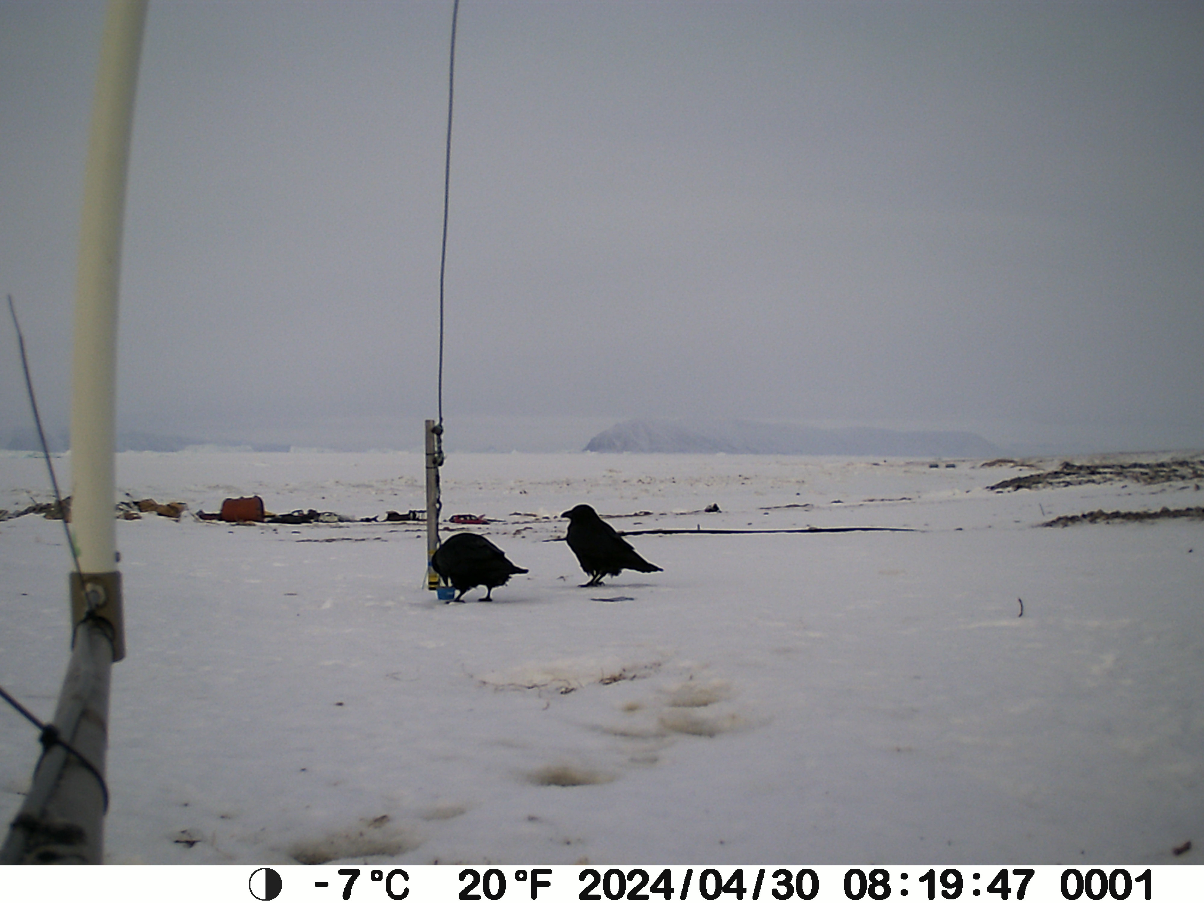
It’s also always fun to check our snowcam – this takes a photo of a stake every 3 hours to monitor the depth of the snow pack, and quite often we get beautiful views and some cheeky ravens hopping past too – I live in hope for an Arctic fox, or even a bear.
Two ravens in the snow, exploring some leftovers apparently.
On the subject of bears, I had heard there were rumours of one near the snow site, but sure enough there were the footprints – rather small and filled in with snow but quite distinctive and heading up towards the ice cap. We shall be extra careful when we go up on to the glacier later this week.
Day 1
We had originally planned terrestrial, glacier and sea ice work, primarily focused on snow processes. The sea ice part though was altered and expanded when the rapid break up in April and again this month was observed. Normally, we’d have a preparation day between arrival and going into the field, but the threat of winds and high temperatures meant we decided not to risk it and we went out straight away on the first full day. Our instincts to just go yesterday turned out to be correct, we had perfect weather and with the help of Qillaq, one of the local hunters we still made it out on to the sea ice. So all is not lost. I woke up this morning to see a wide blue sea just off the last pieces of fast ice on Qaanaaq, so I’m very happy with that decision. Sentinel-2 captured this yesterday while we were out in fact.
It probably looks more dangerous than it is. We were working on the stable fast ice to the east of the big flake, that stretches right into the fjord. The local topography make it very stable and our measurements yesterday confirmed it’s pretty typical for the time of year in thickness, though there was a surprising amount of snow on top, which can actually help to protect the ice from melt at this time of year.
Getting around the coast was surprisingly straightforward, the fast ice has a very stable platform, though some large churned up part of the ice with cracks made for some slightly bumpy manoeuvres to get on and off the stable parts.
Manoeuvring the sled through the coastal zone
The dogs were I think happy when it was over. But in fact it was much more straightforward than I’d feared. The large crack we noticed earlier in the week that opened into a wide lead further extended while we were out, see below, and I woke up this morning to a wide open lagoon. It’s an extraordinarily beautiful place to work and I feel so privileged, especially on days like today when the weather is also being extra nice.
Happy dogs on the way home. Note the large area of open water behind that opened up while we were out.
Work wise it was a successful day, we managed 2 stations, where we did very extensive work. I’d have liked a third but the deep snow made it very heavy and slow going to travel on and in spite of the early start we basically ran out of time and had to return home.
Qillaq and Abraham taking a manual measurement of snow depth and ice thickness next to target for the UAV calibration flights.
We flew the UAV for surface properties, did a lot of snow pits and snow surface properties work, drilled some ice cores (which I will be working on this morning) and even got our loaned EM31 working to do automated ice thickness mapping. We will hopefully start to look at the data later on today to make sure it makes sense before we leave on Thursday.
Our first sea ice core of the season
The reduction in ice means we can actually concentrate on the terrestrial part of the work plan for the rest of the week. And there’s a lot to do!
Last year I set up a semi-permanent snow site to monitor conditions on land through the year. It is going to get a bit of an upgrade this week with some new instruments and of course we need to get the rest of the data downloaded and processed from here too.
I’m writing this from a hotel room in Ilulissat, rather than Qaanaaq where I had intended to be arriving shortly, because our plane has been cancelled due to bad weather (at time of writing the airport was measuring gusts of 14 m/s, so I’m actually quite glad it was cancelled).
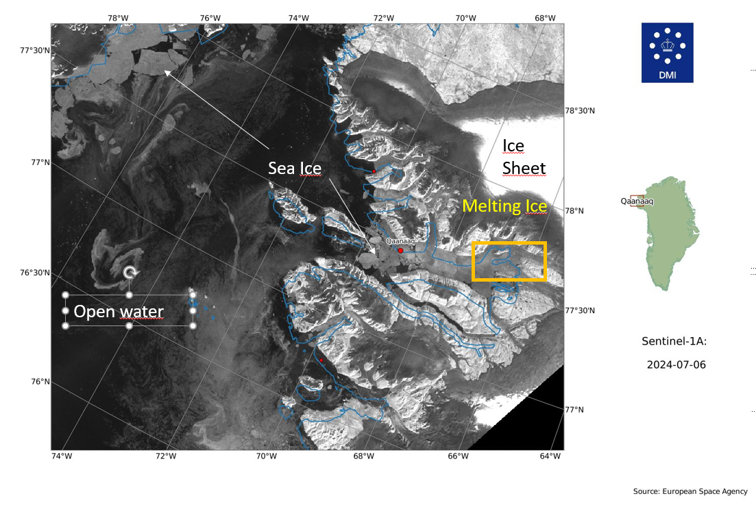
Weather and flight cancellations are an eternal hazard when doing fieldwork in Greenland, but in this case it also means an impact on our planned fieldwork, because the sea ice is falling apart. And rather earlier than usual (though we have not yet done a systematic review to prove this). In fact, part of the reason for coming here in May (instead of my usual March trip) was to investigate an interesting event that happened earlier this spring. In the animation of satellite pictures below you can see the sea ice rather dramatically falling apart in mid-April and then again at the end of April.
The March to May sea ice season from Sentinel 2 in NW Greenland
To understand what is happening and why it’s unusual, first a bit of background. As I have written before, my DMI colleagues have been working up in NW Greenland for about 15 years on a programme of ocean measurements in the fjord (see map below). I joined about 5 years ago, working in the melange zone of the glaciers at the head of Inglefield Bredning (PSA: a paper we recently submitted about this programme will hopefully be online soon). We use the sea ice as highway and stable platform for observations, so it’s pretty important for us and came to the conclusion it wa squite important for some parts of the glaciers too. The local community, with whom we work closely use it also for travelling, hunting and fishing from. It’s extremely important for them.
The region of North West Greenland we’re talking about
Normally there’s pretty thick (~1m) sea ice covering the whole of Inglefield Bredning (Gulf of Inglefield, also known as Kangerlussuaq, but not that one) out to the islands of Qeqertarsuaq and Kiatak. You can seen an example of what this looks like normally in the satellite animation from 2020, which happens to be when my first trip out on to the sea ice in Qaanaaq took place at the end of May and beginning of June. We were actually very lucky, we had great weather, got very close to the ice edge and watched narwhals swimming out in the North Water polynya. (Yes, sometimes I wonder how I managed to get this job too). The animation below is Sentinel-2 images as cloud free as I could find them from that first field season. As you can see, the sea ice already in March was much much more extensive than this year at the same time. And perhaps that is part of the answer.
It’s probably worth pointing out at this stage that although there were some pretty warm (unusually so) spikes in March and April, the sea ice breakup in April was probably largely driven by ocean swell, and perhaps some winds which were strong, though not excessively so as far as we can see in the observations. The latest break-up seems to be driven also by high winds.
Back to our current field season. We had in fact planned a brief trip up here already – I am currently setting up a project looking at snow processes with the team and we had planned to install and test some new instruments and protocol that we hope to use in Antarctica later this year (more on all of that later hopefully). However, as the soon to be published preprint shows, I and the team have developed pretty extensive sea ice interests recently, so this unusual behaviour rather piqued our curiosity.
We have a lot of questions:
Why did it happen this year? Is it really the earliest in the satellite record? What makes the ice vulnerable? Composition, thickness, temperature? Is the ocean driving it or the atmosphere or both (it’s usually both), and what makes this year so unusual? Further down the line, can we model it and use those simulations to understand if this is a single aberration or likely to be more common in the future? And what impact will the earlier breakups have on the ecosystem, the adjacent glaciers and the local community?
Or fieldtrip thus appeared an excellent opportunity to grab some real data on all of these points. Our colleague Henriette Skourup at DTU-Space was kind enough to lend us one of her instruments, which we shipped up last minute to allow us to do an add-on. It is all currently sitting there waiting for us.
Unfortunately the sea ice is not waiting for us, if the photos from my colleague in Qaanaaq, Aksel are anything to go by.
A large and widening crack in the sea ice in front of Qaanaaq. The small objects on the sea ice (fishing gear?) suggest we were not the only ones surprised). Credit: Aksel Ascanius, DMI
The high winds which grounded our plane have also been busy on the sea ice, which is falling apart in the bay with surprising speed as far as I can see. We are still waiting for today’s optical imagery but the quick look from radar based Sentinel-1 suggests cracks widening rapidly as the photo above confirms.
Temperature observations from Qaanaaq airport
With a bit of luck we will get to Qaanaaq on Thursday (immaqa) to see if our sea ice research plan can go ahead. At this stage I rather doubt it. But it will very much depend on the next few hours. The wind speeds are quite high still but the temperature which was well above freezing has now dropped down to just below.
Wind observations from Qaanaaq airport
We are fortunate that we work with local hunters on the sea ice who are immensely experienced. The first rule is always safety first. We do have *a lot* of other work to do and rather fewer days to do it all in, so either way we’ll be busy. Ffor now, it’s keep checking in with the weather, the satellite images and our friends in Qaanaaq and use the time in Ilulissat wisely – in our case, it’s time to write some papers. And one of them is all about sea ice.
To be continued…
All satellite imagery on this page is from the European Space Agency Sentinel-2 mission, processed on the Copernicus EO Browser – a FREE!! and easy to use entry point to use ESA data. Weather observations are from Qaanaaq airport, operated by Mittarfeqarfiit A/S – Grønlands Lufthavne (Greenland Airports) and processed by DMI. It’s actually pretty nice how much high quality data we have access to these days…
This is the first in a two-parter. At this time of year, posts making bold statements about what happened last year and what we plan to do this year start to become prominent. The last few years I have spent a few hours in the first week of January reviewing what worked, what was fun and what was cool, what was awful and what definitely was a waste of time. I’m not honestly sure that any of this is of interest to anyone except me, so read on, but you have been warned..
2024: Themes of this year: Greenland, Machine Learning, people, and big data…
Working with scientists from the Greenland natural resources institute and local hunters on the sea ice.
The final trip was in October for a workshop with scientists in Greenland about climate change impacts in Greenland, the subpolar gyre and AMOC for the UN Ocean decade. It was a memorable meeting for the sheer range and quality of science presented as well as for being stranded in Nuuk by a broken aeroplane in quite ridiculously beautiful weather (I mostly stayed in my hotel room to write the aforementioned paper, sadly. In 2025 I will work on my priorities) .
Apart from fieldwork I have really tried hard on publications this year. I have (like many scientists I suspect), far more data sitting around on hard drives than I have published. It’s a waste and it’s also fun to work on actual data instead of endless emails. This is something I intend to continue focusing on the next few years as well. There is gold in them thar computers…
We had a couple of writing retreats were very successful. These I plan to continue also and the PRECISE project grant is happily flexible enough to do this. I probably achieve as much in terms of data processing and paper writing in 3 focused days as I would in 3 months in the office. It paid off too. I managed to co-author 8 papers published this year (including my first 1st-author paper in ages – a workshop report, but nevertheless it counts.). Some of these are still preprints, so will change, and there are a couple more that have been submitted but are not yet available as preprints. I will submit two more papers in the next 3 weeks as well (1 first author), so January 2025 is going to be the 13th month of 2024 in my mind.
Bootcamps have been a theme the last 3 years, I organised the first in 2022 and so far there have been 4 publications from that first effort. There was another this year in June, ( I have attended them in 2023 and 2024 but was not organising) where we really got going on a project for ESA that I have had my eye on for a while – I hope the publication from that will be ready in the Spring this coming year.
Machine Learning: This was the year I really got machine learning. I’ve been following a graduate course online, and learning from my colleagues and students about implementations. I understand a lot more about the architecture and how to in practice apply neural networks and other techniques like random forests now. This is not before time, as we intend to implement these to contribute to CMIP7 and the next IPCC report. We still have a lot of work to do, but the foundation is laid. And it’s been fun to learn something that, if not exactly new, is a new application of something. In fact the biggest barrier has really been learning new terminology. We have also been fortunate that Eumetsat and the ECMWF have been very helpful in providing us with ML-optimised computer resources to test much of these new models out on. We’re actually running out of resources a bit though, so it’s time to start investigating Lumi, Leonardo and the new Danish centre Gefion to see what we can get out of these.
People: This year our research group has grown with another 2 PhD students, and at the end of the year we also employed a new post-doc. I think it’s large enough now. I’m very aware that if I don’t do my job properly, then not only the research but the people will suffer, so developing people management skills is really important. In any case it’s extremely stimulating to work with such talented young people and I’m really excited to see where the science will take us, given the skills in the team. I hope I have been good enough at managing such a large and young team, but I have my doubts. A focus for 2025 for sure.
Data: This has been the year of big data, not necessarily just for ML purposes but also in the PolarRES project the production and management of an enormous set of future climate projections at very high resolution. More on this anon. Suffice to say, it has taken a lot of my time and mental energy and it’s probably not the most exciting thing to talk about, but we now have 800 Tb of climate simulation data to dig into. I suspect that rewards of this will be coming for years. There has also been a lot of digging into satellite datasets and the bringing together of the two has been very rewarding already. It’s a rich seam, to continue the metaphor, that will be producing scientific gold for many years.
Projects: we have gone in the final year of two projects, PROTECT and PolarRES, both of which will finally end in 2025. We also arrived at the half way point of OCEAN:ICE. So rather than being a year of starts, it has been a year where we have started to prepare for endings – actually this is a fun part of many projects where a lot of the grunt work is out the way and we can start to see what we have actually found out. It can also be a slog of confusing data, writing and editing papers and dealing with h co-author comments. I’ve definitely been in that process this year, hopefully with some of the outputs to come next year…
Proposals: I started 2024 writing a proposal. Colleagues were in 3 different consortia for the same call, alas ours didn’t get funded, but 2 of the others did and will start this year. That is a good result for DMI and our group. I wrote another proposal in the Autumn and contributed to a 4th and finally at the end of the year I heard that both will *likely* be funded (but are currently embargoed and in negotiation, so no more will be said now). It sometimes feels that spending so much time and energy on proposal writing is putting the cart before the horse, but in fact I find proposal writing something akin to brainstorming. It’s essential of course to ensure we can continue to do the science we want, but it can also help us to clarify our ideas and make sure we’re not on the wrong track. It’s also a good way to keep track of what the funders are actually wanting to know and to help us focus on policy relevance.
There was also an incredible number of meetings, reports, milestones and deliverables, but you probably don’t want to hear about that…
Also missing from this summary is personal life, and, well that is not for sharing publically, but suffice to say, I learnt about raising teenagers, I also had some very good times with friends and family, to all of whom I immensely grateful for being a part of my voyages around the sun.
Anyway, reading all that back, I’m not surprised I ended the year exhausted! I am not planning on quite such a slog in future. I should probably pace myself a bit more this year, the plans for which will be the subject of next week’s post.
I’m a co-author on a new paper that has just come out in GRL. It’s based on simulations we did with our collaborators in the PROTECT project on sea level contributions from the cryosphere. What Glaude et al shows is that, to quote the first of the 3 key points:
“With identical forcing, Greenland Ice Sheet surface mass balance from 3 regional climate models shows a two-fold difference by 2100”
In perhaps more familiar terms, if you run 3 regional climate models (that is a climate model run only over a small part of the world, in this case Greenland) with identical data feeding in from the same global climate model around the edges, you will get 3 quite different futures. Below you can see how the 3 different models think the ice sheet will look on average between 2080 and 2100. The model on the right, HIRHAM5 is our old and now retired RCM. It has a much smaller accumulation area left by the end of the century than the other two, which have much more intense melt going on in the margins.
Greenland Ice Sheet annual surface mass balance (a, b, c, 2080–2099 average) and annual surface mass balance anomaly (d, e, f, 2080–2099 average relative to 1980–1999) [mm WE/yr]. From left to right, RACMO (a and d), MAR (b and e), and HIRHAM (c and f). The equilibrium line (SMB = 0) is displayed as a solid black line in (d-f). Glaude et al., 2024, GRL.
In fact, by the end of the century, although the maps above seem to show HIRHAM having much more melt, there is in fact more runoff from the MAR model, because of this intense melt.
Spatially aggregated annual GrIS SMB anomalies (a), total precipitation (PP, b), and runoff (RU, c) [Gt/yr]. The solid lines represent the anomalies using a 5-year moving average, while the transparent lines display the unfiltered model output.
The surface mass balance (SMB) at the present day is in fact positive. This often surprises people, but SMB as the name suggests, only describes surface processes. Ice sheets can (and do) also lose a lot of ice by calving and subglacial and submarine melt. As SMB should balance everything if a glacier is to remain stable or even grow, present day SMB is usually 300 to 400 GT positive at the end of each year, and even so the Greenland ice sheet loses, net around 270Gt per year.
Our work here shows that, at least under this pathway, not only does SMB become net negative in itself by the middle of this century, there are significant differences in SMB projections between the estimates of how negative it will be, between the three RCMs. The global model we used, CESM2 under the high-end SSP5-8.5 scenario, is famously a warm scenario, but our estimated end of the century SMBs are extraordinary : (−964, −1735, and −1698 Gt per year, respectively, for 2080–2099). As I’ve discussed previously, one gigatonne is a cubic kilometre of water, 360Gt is roughly 1mm global mean sea level rise. (Though note your local sea level rise is *definitely* not the same as global average!) Even the lowest estimate here the is giving around 3 mm of global average sea level rise from surface melt and runoff *alone* by the end of this century each year. That’s pretty close to the modern day observed sea level rise from all sources.
And this is in spite of the fact that at the present day, the 3 models are rather similar in their estimates of SMB. The Devil is as usual in the details.
We attribute these startling divergences in the end of the century results to small differences in 1) the way melt water is generated, due to the albedo scheme (that is how the ice sheet surface reflects incoming energy); 2) but also due to the cloud parameters that control long-wave radiation at the surface, which again can promote or suppress melting. (We really need to know how much liquid water or ice there are in clouds, as this paper also emphasises in Antarctica); and 3) mainly down to the way liquid water that percolates down from the surface is handled in the snow pack. That is, how much air there is in the snowpack, how warm the snow is and how much refreezing can occur to buffer that melt.
The problem is that all of these processes happen at very small scales, from the mm (snow grains and air content), to the micron scale (cloud microphysics). That means that even in high (~5km) resolution regional models, we need to use parameterisations (approximations that generalise small scale processes over larger spatial and/or time scales). Small differences between these parameterisations add up over many decades. Essentially, much like the famous butterfly flapping its wings in Panama and causing a hurricane in Florida, the way mixed phase clouds produce a mix of water vapour and ice over an ice surface might ultimately determine how fast Miami will sink beneath the waves.
More data would certainly help to refine these parameterisations. The main scheme to work out how much liquid can percolate into snow was originally based on work by the US Army engineers in the 1970s. More field data with different types of snow would surely help refine these. Satellite data will be massively helpful, if we can smoothe out some wrinkles in how clouds (there they are again) affect surface reflectivity.
These 3 different types of processes also interact with each other in quite complex ways and ultimately affect how much runoff is generated as well as the size of the runoff zone in each model. So integration of many different types of observations is crucial.
“Different runoff projections stem from substantial discrepancies in projected ablation zone expansion, and reciprocally” as we put it in Glaude et al., 2024.
The timing and magnitude of the expansion of the runoff zone is quite different between the models, but all of them show a very consistent increase in melt and runoff over the next 80 years.
It’s probably also important to understand a couple of key points:
Firstly we ran a very high emissions pathway: SSP5-85 is probably not representative of the path we will follow in emissions (at least I hope not), but in this study we wanted to address the spread on different model estimates. And this is a way to get a good check on the sensitivity.
Secondly, the ice sheet mask and topography in these runs is kept fixed all the way through the century. This means we do not account for any elevation feedbacks (as the ice sheet gets lower because of melt, a larger area becomes vulnerable to melt because it’s lower and thus warmer), but we also don’t account for ice that has basically melted away no longer contributing to calculated runoff later in the century. Ice sheet dynamics are also not factored in.
Finally, we ran different resolution models, and that can have an impact particularly on precipitation and is one of the reasons why the new models we developed and have run in PolarRES (and which are now being analysed), have used a much more consistent set-up.
The 3 models we used, MAR, RACMO and HIRHAM have all been used in many different studies over both Greenland and Antarctica, but we haven’t really done a systematic comparison of future projections before. I think this work shows we need to get better at doing this to capture the uncertainty in the spread, especially when you consider that we’re now looking at using these models as training datasets for AI applications: training on each one of these models would give quite different results long-term. We need to think about how to both improve numerical models and capture that spread better. But ultimately, it’s how fast we can reduce greenhouse gas emissions and bend the carbon dioxide curve down that will determine how much of Greenland we will lose, and how quickly.
All data and model output from these simulations is available to download on our servers (we’re transitioning to a new one download.dmi.dk, not everything has been moved there yet). We also of course have data over land points and the surrounding seas, and we’ve run many more global climate models through the regional system to get high resolution (5km!) climate data also looking at different emissions pathways, if you’re interested in looking at, analysing or using any of this data – get in touch!
My warmest thanks to Quentin Glaude who led this analysis and special thanks to our colleagues in the Netherlands, France and Belgium for running these models and contributing to the paper analysis. Clearly, we have much work to do to get better at this ahead of CMIP7.
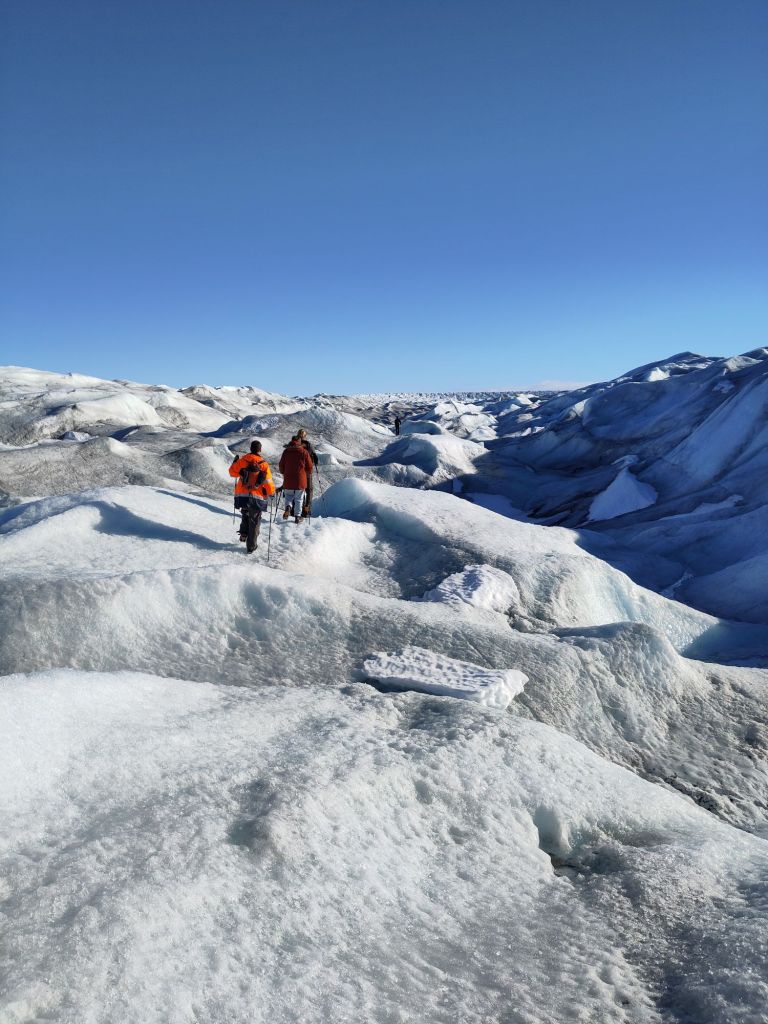
Group field trip the Greenland ice sheet: it’s important to see what you’re modelling actually looks like….
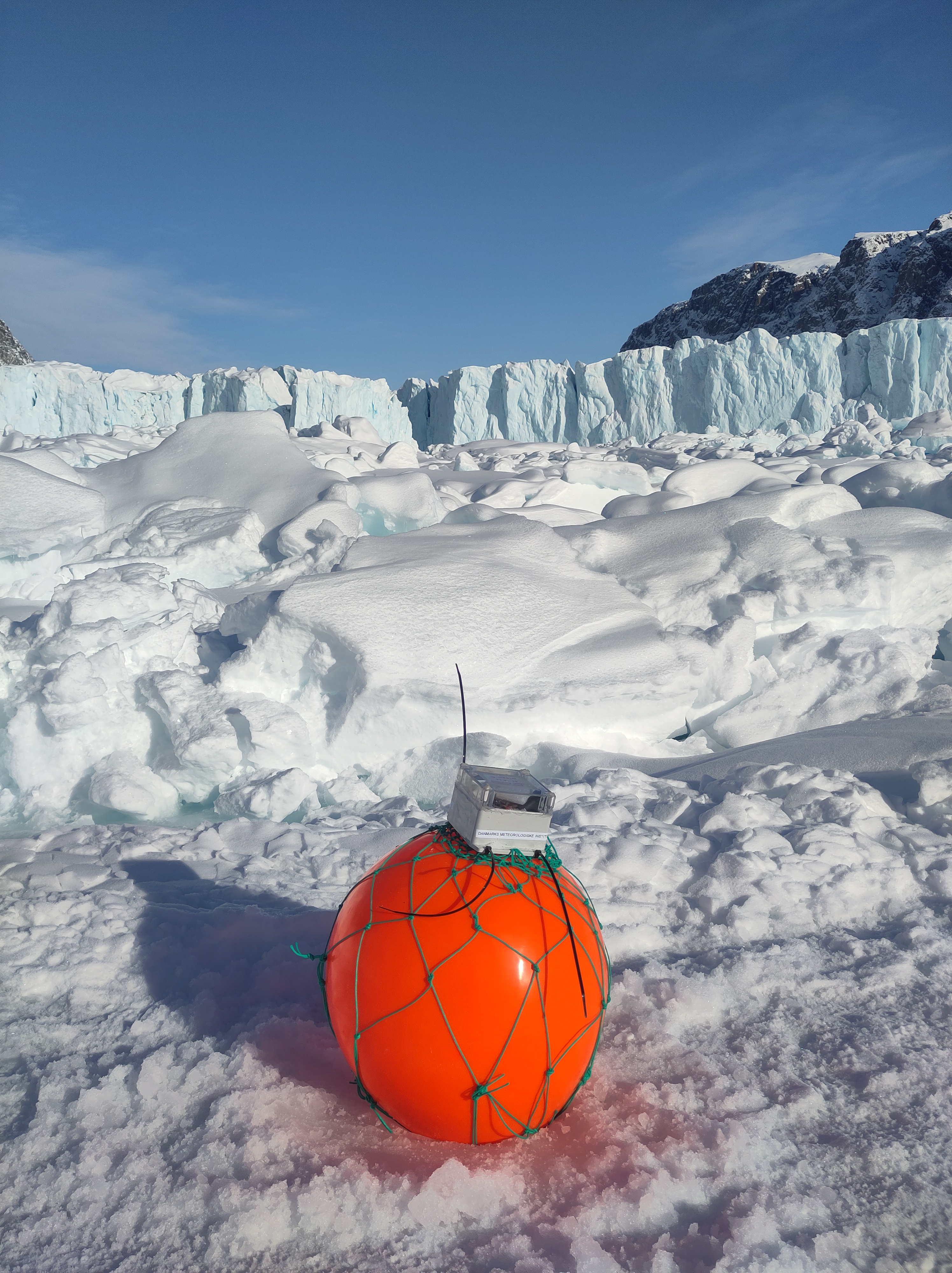
Way back in the mists of time, that is, early April, I and colleagues deployed some instruments on the sea ice in front of a number of glaciers in Northern Greenland, which I wrote a little bit about here.
Trusted global GPS tracker buoy
Open met buoy
Since then I’ve mostly been letting them get on with reporting their data back and occasionally checking on the satellite imagery to see how it’s looking in their surroundings.
It was about -30C and very cold when I left them out, so it’s sometimes quite hard to visualise just how much things will change over only a few months and to remember that at some point, they’ll need collecting
After a fairly melty start (yes, that is actually a technical term) to July, particularly in the northern part of the ice sheet (which you can see on the polarportal, see also below right) it’s time to start anticipating their collection.
We have a lot of advantages when it comes to coordinating this kind of project now, compared to the bad old days when imagery and communication were both scarce and expensive
For starters, there is Sentinel Hub’s EO browser, a course in which should be a requirement for every earth science adjacent subject in my opinion. EO Browser produces superb pre-processed imagery for free, such as this one, from the European Space Agency’s Sentinel-2 satellite yesterday
As you can see, the sea ice is still there but fracturing and patches of open water (in blue green) are now becoming visible.
Sentinel 2 satellite image processed on EO browser showing sea ice and ice bergs in front of Tracy and Farquhar glaciers.
If you’re out and about and only have your phone, there is also the excellent snapplanet.io app on your smartphone, with which you can create instagram ready snapshots of the planet or even animated gifs, with high resolution imagery a link away…
Now that’s what I call a fun social media* application…
Animated gif of satellite images showing the front of Heilprin glacier with icebergs and landfast sea ice.
Anyway, back to the break up. Every year, the sea ice forms in the fjord from October/November onwards, by December it’s often thick enough to travel on and then from April it starts to thin and melt and by late June large cracks are starting to form, allowing the surface meltwater to drain through. For a look at what happens if you get a large amount of melt from, say, a foehn wind, before the cracks start to open up, see this iconic photo taken by my colleague Steffen Olsen in 2019.
An extremely rare event, that nevertheless went viral
The other advantage we have working in this fjord is our collaboration with the local hunters and fishers. In winter they use dog sleds for hunting and accessing fishing sites, and to take us and our equipment out on to the ice. In summer, they are primarily using boats for fishing, hunting narwhal and, hopefully, collecting our equipment! Our brilliant DMI colleague Aksel who lives and works in the local settlement is also a huge help in assisting with communication and generally being able to get hold of things and people when asked.
Winter travel
We offer a reward for each buoy that is found and brought back to our base in Qaanaaq, so many of them in fact make their own way home. But we also work with our friends on a kind of remote treasure hunt, challenge Anneka style, with someone at home watching their positions come in via the satellite transmissions and sending updated information via sms to an iridium phone to the hunters on the boat…
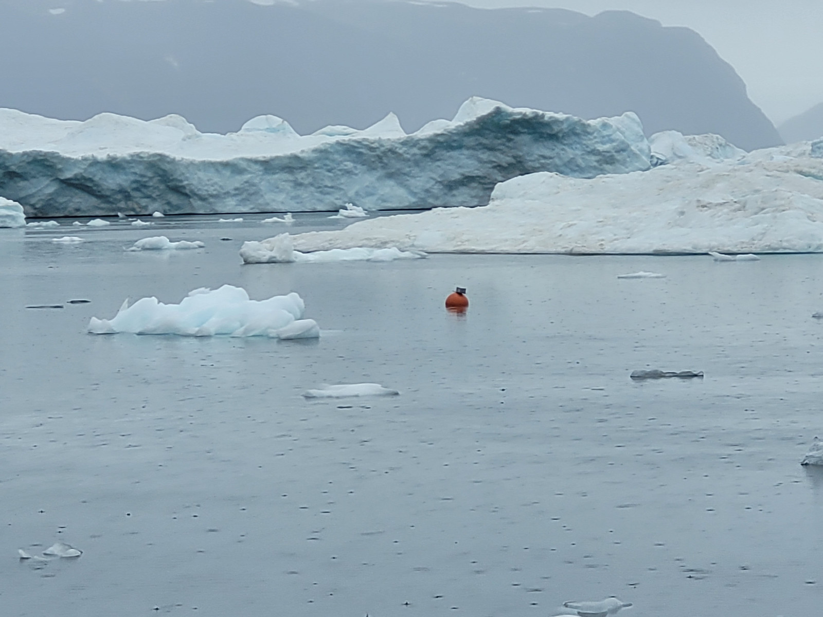
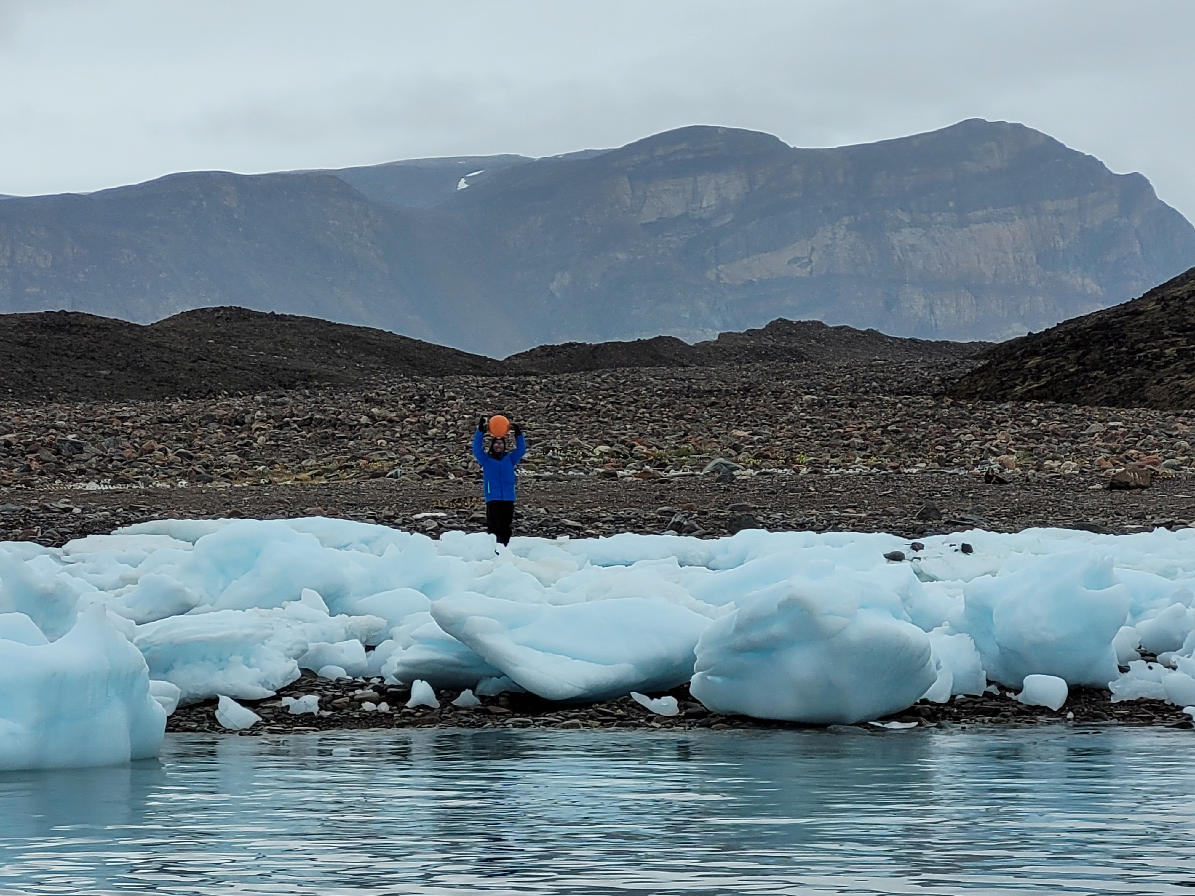
I’m told it’s tremendous fun, with sharp eyes required, as even a bright orange plastic globe can be challenging to spot.
A floating trusted buoy in 2022.
I’ve never participated in this treasure hunt myself sadly, on land we generally see something like a spaghetti of arrows and spots via the Trusted global web api:
GPS positions from a trusted buoy.
We then have to try and superimpose these movements on the latest satellite images to work out if the buoy is floating or not, and then check to see if there is sufficient open water for a collection. Naturally working with local knowledge for this part is also absolutely vital.
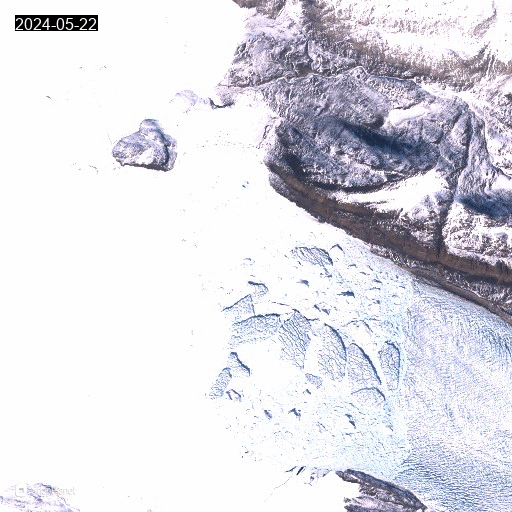
One of our buoys is found…
The latest satellite images look like the ice has already broken up into large flakes close to Qaanaaq. I’ve annotated the Sentinel-1 image below as it is from a radar satellite that can see through clouds and the images can be a bit confusing if you’re not used to looking at them.
The scale of the massive melt on the ice sheet from the last few days is clearly visible in the dark grey rim on the glaciers. The open sea water is black and the sea ice shows up as geometric greys. This one is downloaded from the automatic archive my colleagues at DMI maintain around the whole coast of Greenland. It can be a handy quick check too.
Annotated satellite image of Kangerlussuaq/Inglefield Bredning (Gulf of Inglefield) fjord. The orange box shows where our study glaciers are located.
So, although the ice is starting to break up it’s at the tricky stage where it’s far from navigable by dog sled and certainly too difficult for boats, so it’s not quite the time to send out hunting parties for GNSS buoys.
It also means that when I go on holiday next week, I will not be quite leaving all this behind. I and my colleague in this project will be monitoring the movements of the buoys and the satellite pictures, as well as relying on our friends in the local community to let us know how the ice is looking and if they can get out to rescue our brave little sensors.
In the mean time I have plenty of data to start analysing and writing up. As ever massive thanks to the people of Qaanaaq and my cool colleagues for putting up with me and our GPS buoys. We hope to submit our first paper pretty soon..
Hopefully I’ll soon be able to look at a map like this one to see where they are (note that the precision on these buoy positions isn’t great, probabaly because they were thenbeing stored in a metal container).
*Yes, I’m probably a nerd. I’m a lot of fun** at parties too though.
Icebergs in Ilulissat drift around the bay, sometimes fast, sometimes slow, sometimes they don’t move at all. They are drenched in the beautiful but sometimes stark light of the polar day. It’s scientifically interesting to watch them and speculate on their past trajectory and their likely future. It’s also extremely beautiful.
I’m once more on my way north to Qaanaaq, but this time I’ve been lucky enough to be able to enjoy some days off in Ilulissat. It’s an astonishing beautiful place, famous for the icebergs that come pouring out of the Ilulissat ice fjord just round the corner.
Normally, we’re only in town for one night as we have to switch planes to get to our field sites and this requires an overnight stay so it has been brilliant to be able to use a little holiday here.
Panorama over the bay in Ilulissat on a sunny evening
I have been using the time to work on some papers and try to clear some of the back log of reports and emails, but there has at least been some time for a couple of hikes in the back country nearby. I could post several hundred photos of icebergs and other magnificent views, but I was struck by the movement of icebergs in the bay outside my window while I was working yesterday.
Sometimes the big bergs seemed to move more, sometimes they seem stuck. I wanted to check this so I set up a time lapse on my tablet in the window of the guest house I’m staying in overnight (bearing in mind it’s the Polar Day so doesn’t actually get dark). I think it actually ran out of power before covering the full six hours I set it up for, so I’m now trying a full day. However, it was enough to show my perception was basically right and I have come to the conclusion the changing movement is related to the tides.
This is also a bit of an excuse to play around with video editing a little, in this case I’m trying out canva, and to advertise my peertube account @icesheets_climate on TILvids.com.
As I’ve alluded to before, I’m trying out the non-corporate social media fediverse and it’s actually quite fun, though the videos are a bit time-consuming so I’m not quite sure how regularly I will manage to post these on my channel, but the clue is in the name on what most of them are about I guess…
Another iceberg near Ilulissat, this time one we visited by boat…
But I have gratuitously many photos on my pixelfed account and no doubt more to come. I’m also planning some icebreaker shorts describing different elements of the environment that I’m working on. We’ll have to see how much time I have to actually get those finished, they typically take a while!
Of course, these are not just pretty pictures – I have a professional interest in icebergs – my PhD was about ice fracture and applying models of crevasse formation to describe a new parameterisation of calving. One of the projects I’m working on in northern Greenland, (funded by the danish state through the National Centre for Climate Research, NCKF) is also focused on calving processes, and specifically the role of ice melange in the system. In fact, one of the papers I’ve been working on this week analyses those iceberg related datasets. It’s immensely valuable and rare that I have the opportunity to be able to focus on the process in the field at the same time as writing the paper.
I have 2 more days in Ilulissat, so no doubt there will be more walks around town and more iceberg photos, but I have sent the iceberg paper back to my co-authors now, so it’s time to focus on a new paper – and the climate of the polar regions in the future.
I’m lifting my head from the semi-organised chaos that is my office, my home office, our family basement and the office workshop to write a quick post. This might be for reasons of despairing procrastination.
The reason for the chaos is that fieldwork season has come round again and on Friday I and my DMI colleague Steffen will be off to Northern Greenland once again. I’ll try to post a few photos to pixelfed (and perhaps even Instagram, though I swore off Meta products after the Brexit fiasco).
This year my focus is again on the melange zone and we’ll be placing our instruments out to record the break-up of the fast ice. I also hope to get time to establish a new snow measurement programme – which I partly piloted last year. However, we will only be 2 scientists instead of the team of 4 this year, so this may have to wait until the second fieldwork period we have planned in early June (when the sea ice starts to break up). We are fortunate indeed that the local hunters, who still live a semi-subsistence lifestyle, are both incredibly competent and helpful and willing and eager to help when we go out on fieldwork.
Last year was a test of concept, and noone was more astonished than I was that the final set up not only survived the ice break up and floated safely down the fjord, we also managed to retrieve them and I hope they are waiting patiently in Qaanaaq so I can reprogramme and redeploy this year.
I wrote this piece on our work last year, promising a whole load of posts I didn’t end up having time to write. Sadly even my lego scientists never got an update. So instead of promising a whole lot of new posts, let me know what you’d like to see and read about either in the comments here or on my mastodon feed, and I’ll try to make some time to answer one or two of them while we go.
The area we travel to is going through very rapid changes now – not just climatic and environmental, but, perhaps even higher impact, social and cultural. I am privileged to be abel to witness it and we try hard to leave as little impact as possible.
At this stage it’s hard to imagine I’ll ever be ready to leave, but the clock is ticking down..
I’ve explained several times in the course of media comments that, when it comes to the sea level rise that you experience, it really matters where the water comes from. This point still seems to cause confusion so I’ve written a super fast post on it.
Waves from the Storm Surge that hit Denmark in October 2023 credit: Sebastian Pelt
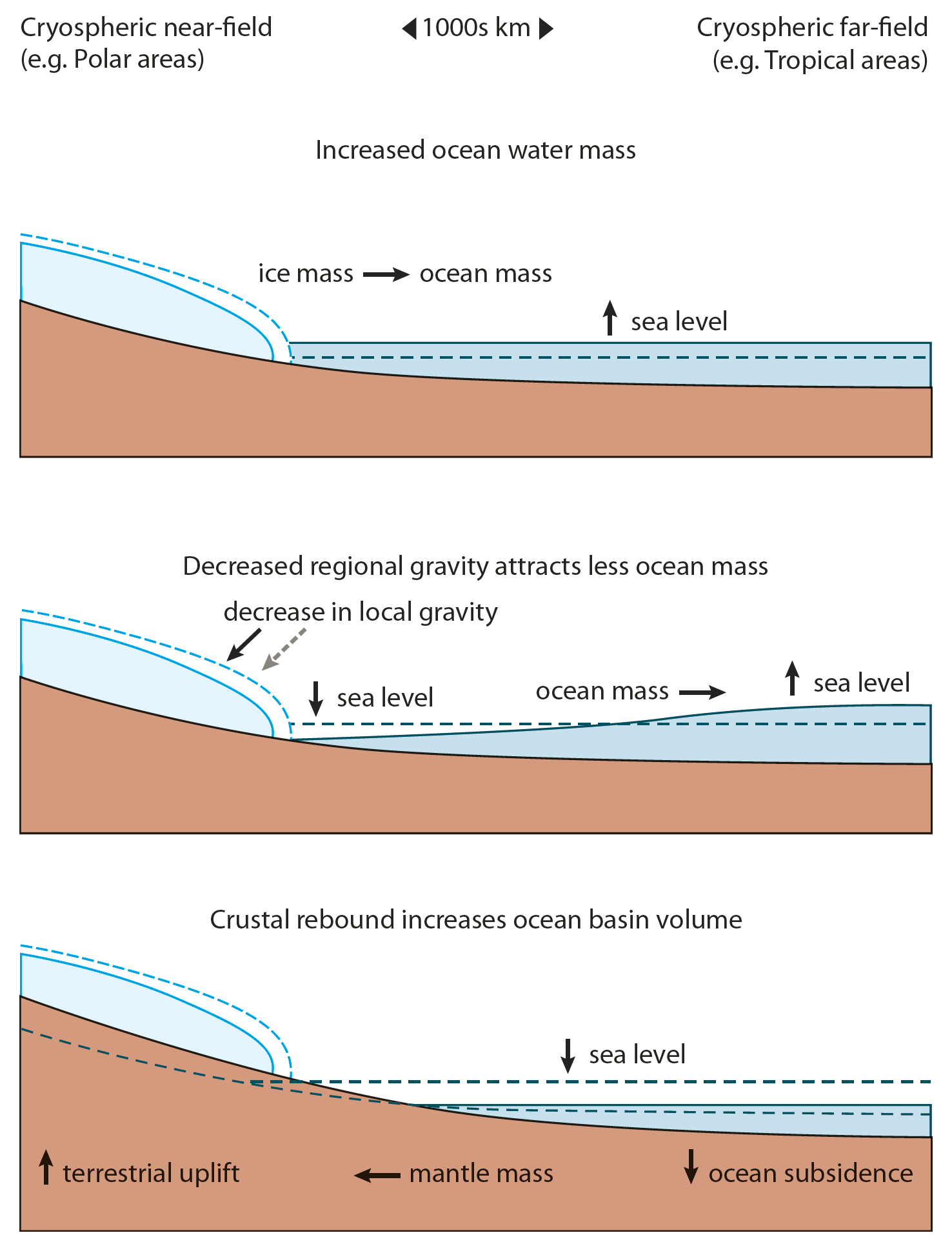
We very often talk about a metre or two of sea level rise by the end of the century, but in general that refers to global average sea level. And much like a global mean temperature rise doesn’t tell you very much about the kind of temperature changes you will experience in your location due to weather or climate, global mean sea level is also not very informative when talking about preparing your local community for sea level rise. There are other local factors that are important, (see below), but here I’m going to mostly focus on gravity.
Imagine that sea level is more or less stable around the earth (which it was, more or less, before the start of the twentieth century). Just like the moon causes tides because its gravity exerts a pull on the oceans, the ice sheets are large masses and their gravity also attracts ocean water, so the average sea level is higher closer to Greenland and to Antarctica. But there is only a finite volume of water in the oceans, so a higher sea level close to the ice sheets means lower sea levels further away in the tropics for example.
As the ice sheet melts and gets smaller, its gravitational pull becomes smaller so the average height of the sea around Greenland and Antarctica is lower than it was before, but the water gets redistributed around the earth until it is in equilibrium with the gravitational pull of the ice sheets again. The sea level in other places is therefore much higher than it would have been without that gravitational effect.
And in general, the further away from an ice mass you are, the more these gravitational processes affect your local sea level change. In Northern Europe, it often surprises people (also here in Denmark) to learn that while Greenland has a small influence on our local sea level, it’s not very much because we live relatively close to it, however the loss of ice from Antarctica is much more important in affecting our local sea level rise.
Currently, most of the ice contributing to sea level is from the small glaciers around the world, and here too there is an effect. The melt of Alaska and the Andes are more important to our sea level than the Alps or Norwegian glaciers because we are far from the American glaciers but close to the European ones.
This figure below illustrates the processes:
Processes important for local sea level include changes in land height as ice melts but also the redistribution of water as the gravitational attraction of the ice sheets is reduced. The schematic representation is from the Arctic assessment SWIPA report Figure 9.1 from SWIPA 2017
This is partly why the EU funded PROTECT project on cryosphere contributions to sea level rise, which I am currently working on, has an emphasis on the science to policymakers pipeline. We describe the whole project in this Frontiers paper, which includes a graphic explaining what affects your local sea level.
As you can see, it very much depends on what time and spatial scale you’re looking at, with the two ice sheets affecting sea level on the longest time scales.
Figure 1 from Durand et al., 2021 Illustration of the processes that contribute to sea level change with respect to their temporal and spatial scales. These cover local and short term effects like storm surges, waves and tides to global and long-term changes due to the melting of ice sheets.
In the course of the project some of the partners have produced this excellent policy briefing, which should really be compulsory for anyone interested in coastal developments over the next decades to centuries. The most important points are worth highlighting here:
We expect that 2m of global mean sea level rise is more or less baked in, it will be very difficult to avoid this, even with dramatic reductions in greenhouse gas emissions. But the timescale, as in when that figure will be reached, could be anything from the next hundred years to the next thousand.
Figure from PROTECT policy briefing showing how the time when average global sea level reaches 2m is strongly dependend on emissions pathway – but also that different parts of the world will reach 2m of sea level rise at very different times, with the tropics and low latitudes in general getting there first.
What the map shows is that the timing at which any individual place on earth reaches 2 m is strongly dependent on where on earth it is. In general lower latitudes close to the equator will get to 2m before higher latitudes, and while there are ocean circulation and other processes that are important here – to a large extent your local sea level is controlled by how close to the ice sheets you are and how quickly those ice sheets will lose their ice.
There are other processes that are important – especially locally, including how much the land you are on is rising or sinking, as well as changes in ocean and atmosphere circulation. I may write about these a bit more later.
Feel free to comment or ask questions in the comments below or you can catch me on mastodon:
Hands-up who is looking for a new and very cool job in ice sheet and climate modelling and developing new machine learning tools?
REMINDER: 4 days left to apply for this PhD position with me at DMI looking at Antarctic Ice Sheet mass budget processes and developing new Machine Learning models and processes.
UPDATE 2: The PhD position on Antarctica is now live here. Deadline for Applications 18th February!
UPDATE: It’s not technically a PRECISE job, but if you’re a student in Copenhagen and are looking for a part-time study job (Note that this is a specific limited hours job-type for students in higher education in Dnmark) , DMI have got 2 positions open right now, at least one of which will be dedicated to very related work – namely working out how well climate and ice sheet models work when compared with satellite data. It’s part of a European Space Agency funded project that I and my ace colleague Shuting Yang, PI on the new TipESM project, are running. Apply. Apply. Apply…
This is a quick post to announce that our recruitment drive is now open. We’re split across three institutes. We are two in Copenhagen, ourselves at DMI and the Niels Bohr Institute at the University of Copenhagen, and then the University of Northumbria in Newcastle, UK.
The PI at the Niels Bohr Institute is the supremely talented Professor Christine Hvidberg, aided by material scientist and head of the institute, Joachim Mathiesen. I am leading for DMI, and the Northumbria work is led by Professor Hilmar Gudmundsson. We are also very fortunate to have the talents of Aslak Grindsted, Helle Schmidt, Nicolas Rathmann and Nicolaj Hansen already on board.
The project is already very cohesive between institutes, we’ve been working together for some time already and know each other well.
We have a good budget for travel and exchanges between groups, workshops, symposia, summer schools and the like, but perhaps more importantly, all the positions are focused at the very cutting edge (apologies for the cliche) of climate and ice sheet modelling. We are developing not just existing models and new ways to parameterise physical processes, but we also want to focus on machine learning to incorporate new processes, speed-up the production of projections for sea level rise, not forgetting an active interface with the primary stakeholders who will need to use the outcomes of the project to prepare society for the coming changes.
There’s also a healthy fieldwork component (particularly in Greenland, I don’t rule out Antarctica either), and if you’re that way inclined, some ice core isotope work too. So, if you’re looking for a new direction, feel free to give me a shout. I’m happy to talk further.
Links to all the openings, will be updated as they come out, these are currently open and have deadlines at the end of January: