I was going to blog about this cool new paper that my colleagues at DMI have produced, but John Kennedy has as always done such a good job I will just point you over there…
Wondering whether a warm bias in the Arctic in ERA5 affects our estimates of global temperature change.
I’ve explained several times in the course of media comments that, when it comes to the sea level rise that you experience, it really matters where the water comes from. This point still seems to cause confusion so I’ve written a super fast post on it.
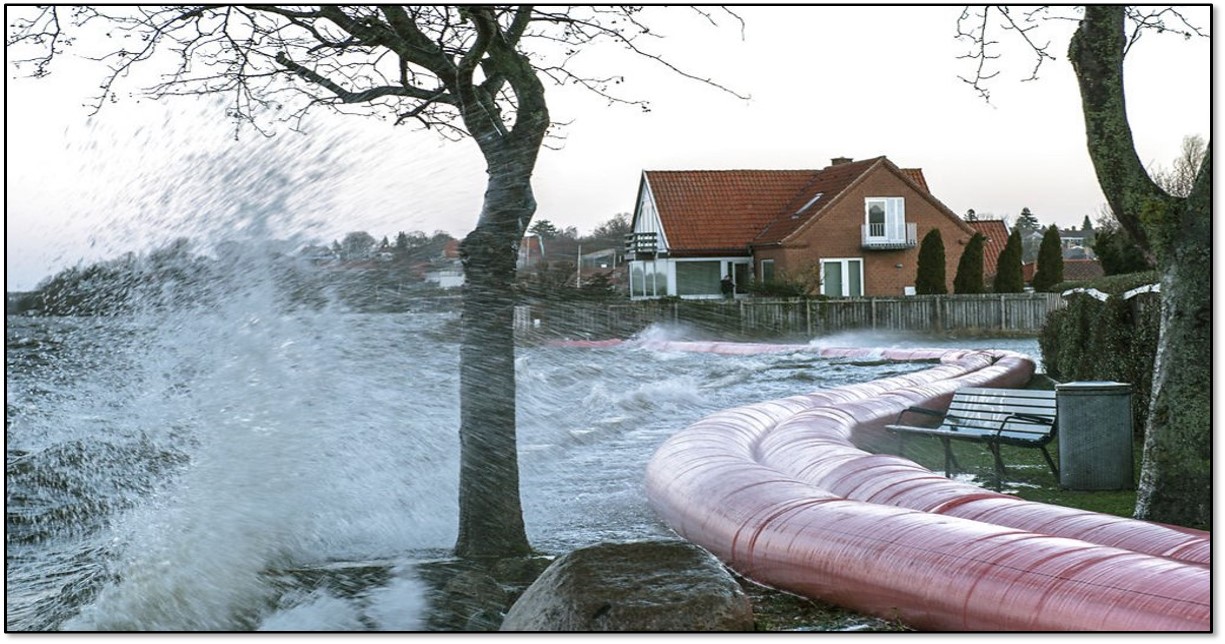
Waves from the Storm Surge that hit Denmark in October 2023 credit: Sebastian Pelt
We very often talk about a metre or two of sea level rise by the end of the century, but in general that refers to global average sea level. And much like a global mean temperature rise doesn’t tell you very much about the kind of temperature changes you will experience in your location due to weather or climate, global mean sea level is also not very informative when talking about preparing your local community for sea level rise. There are other local factors that are important, (see below), but here I’m going to mostly focus on gravity.
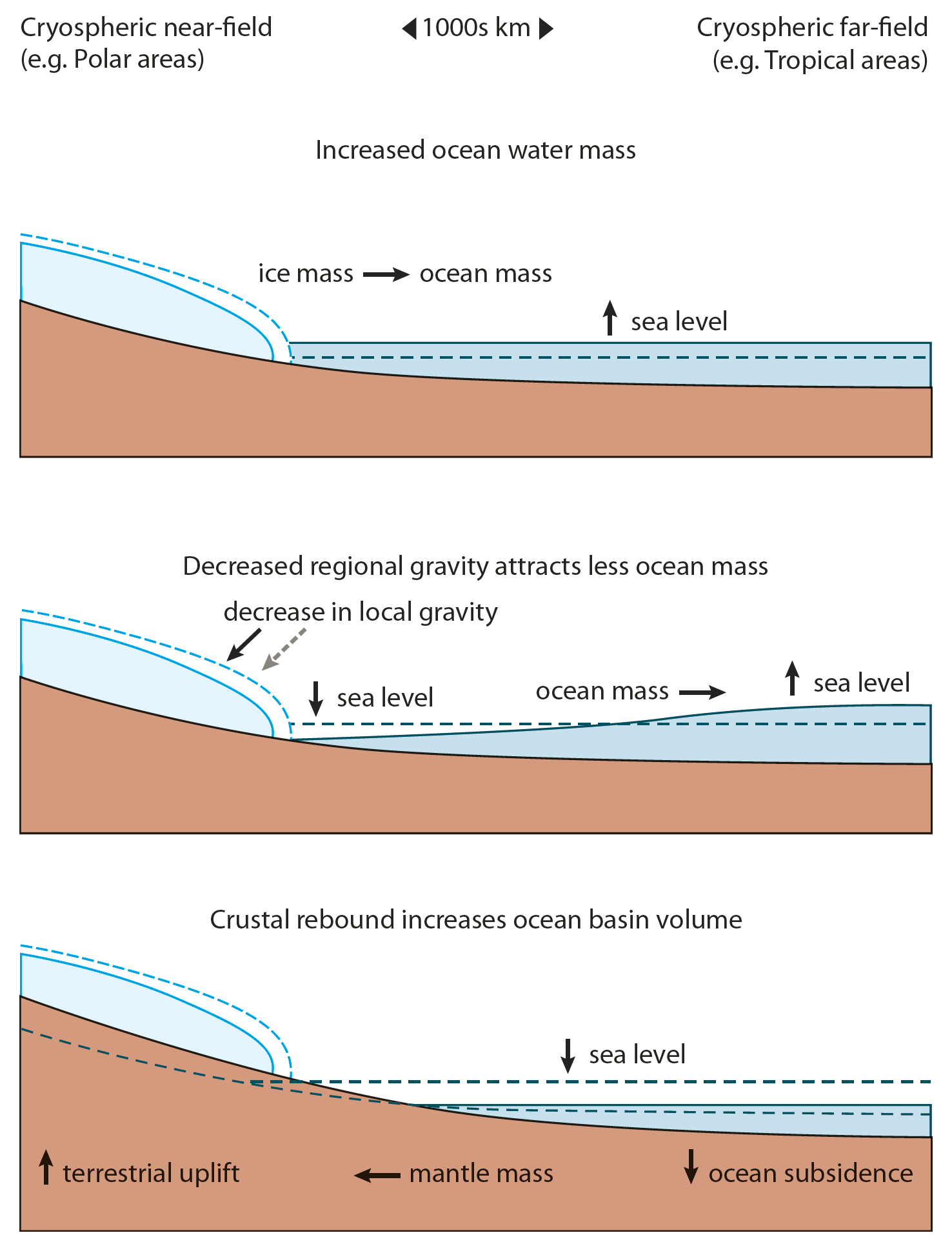
Imagine that sea level is more or less stable around the earth (which it was, more or less, before the start of the twentieth century). Just like the moon causes tides because its gravity exerts a pull on the oceans, the ice sheets are large masses and their gravity also attracts ocean water, so the average sea level is higher closer to Greenland and to Antarctica. But there is only a finite volume of water in the oceans, so a higher sea level close to the ice sheets means lower sea levels further away in the tropics for example.
As the ice sheet melts and gets smaller, its gravitational pull becomes smaller so the average height of the sea around Greenland and Antarctica is lower than it was before, but the water gets redistributed around the earth until it is in equilibrium with the gravitational pull of the ice sheets again. The sea level in other places is therefore much higher than it would have been without that gravitational effect.
And in general, the further away from an ice mass you are, the more these gravitational processes affect your local sea level change. In Northern Europe, it often surprises people (also here in Denmark) to learn that while Greenland has a small influence on our local sea level, it’s not very much because we live relatively close to it, however the loss of ice from Antarctica is much more important in affecting our local sea level rise.
Currently, most of the ice contributing to sea level is from the small glaciers around the world, and here too there is an effect. The melt of Alaska and the Andes are more important to our sea level than the Alps or Norwegian glaciers because we are far from the American glaciers but close to the European ones.
This figure below illustrates the processes:
Processes important for local sea level include changes in land height as ice melts but also the redistribution of water as the gravitational attraction of the ice sheets is reduced. The schematic representation is from the Arctic assessment SWIPA report Figure 9.1 from SWIPA 2017
This is partly why the EU funded PROTECT project on cryosphere contributions to sea level rise, which I am currently working on, has an emphasis on the science to policymakers pipeline. We describe the whole project in this Frontiers paper, which includes a graphic explaining what affects your local sea level.
As you can see, it very much depends on what time and spatial scale you’re looking at, with the two ice sheets affecting sea level on the longest time scales.
Figure 1 from Durand et al., 2021 Illustration of the processes that contribute to sea level change with respect to their temporal and spatial scales. These cover local and short term effects like storm surges, waves and tides to global and long-term changes due to the melting of ice sheets.
In the course of the project some of the partners have produced this excellent policy briefing, which should really be compulsory for anyone interested in coastal developments over the next decades to centuries. The most important points are worth highlighting here:
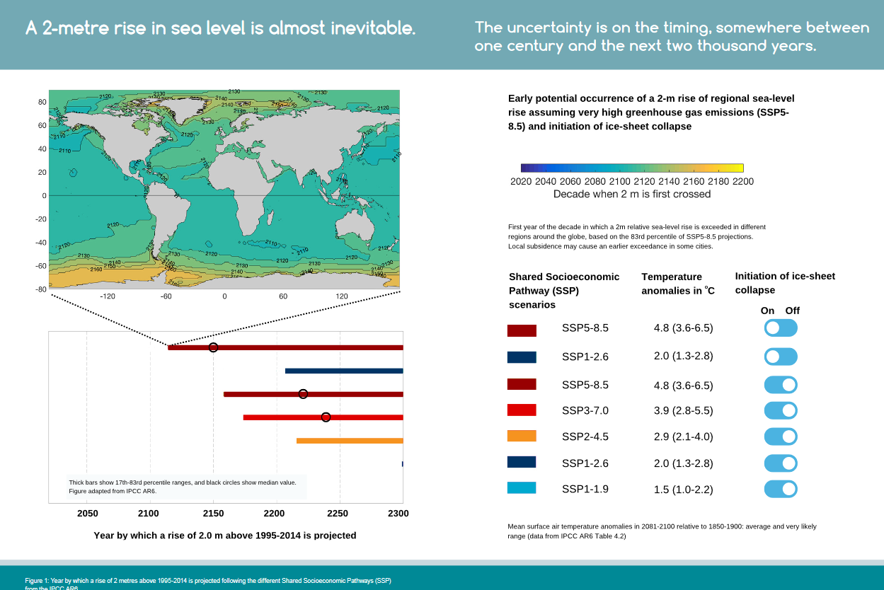
We expect that 2m of global mean sea level rise is more or less baked in, it will be very difficult to avoid this, even with dramatic reductions in greenhouse gas emissions. But the timescale, as in when that figure will be reached, could be anything from the next hundred years to the next thousand.
Figure from PROTECT policy briefing showing how the time when average global sea level reaches 2m is strongly dependend on emissions pathway – but also that different parts of the world will reach 2m of sea level rise at very different times, with the tropics and low latitudes in general getting there first.
What the map shows is that the timing at which any individual place on earth reaches 2 m is strongly dependent on where on earth it is. In general lower latitudes close to the equator will get to 2m before higher latitudes, and while there are ocean circulation and other processes that are important here – to a large extent your local sea level is controlled by how close to the ice sheets you are and how quickly those ice sheets will lose their ice.
There are other processes that are important – especially locally, including how much the land you are on is rising or sinking, as well as changes in ocean and atmosphere circulation. I may write about these a bit more later.
Feel free to comment or ask questions in the comments below or you can catch me on mastodon:
Hands-up who is looking for a new and very cool job in ice sheet and climate modelling and developing new machine learning tools?
REMINDER: 4 days left to apply for this PhD position with me at DMI looking at Antarctic Ice Sheet mass budget processes and developing new Machine Learning models and processes.
UPDATE 2: The PhD position on Antarctica is now live here. Deadline for Applications 18th February!
UPDATE: It’s not technically a PRECISE job, but if you’re a student in Copenhagen and are looking for a part-time study job (Note that this is a specific limited hours job-type for students in higher education in Dnmark) , DMI have got 2 positions open right now, at least one of which will be dedicated to very related work – namely working out how well climate and ice sheet models work when compared with satellite data. It’s part of a European Space Agency funded project that I and my ace colleague Shuting Yang, PI on the new TipESM project, are running. Apply. Apply. Apply…
This is a quick post to announce that our recruitment drive is now open. We’re split across three institutes. We are two in Copenhagen, ourselves at DMI and the Niels Bohr Institute at the University of Copenhagen, and then the University of Northumbria in Newcastle, UK.
The PI at the Niels Bohr Institute is the supremely talented Professor Christine Hvidberg, aided by material scientist and head of the institute, Joachim Mathiesen. I am leading for DMI, and the Northumbria work is led by Professor Hilmar Gudmundsson. We are also very fortunate to have the talents of Aslak Grindsted, Helle Schmidt, Nicolas Rathmann and Nicolaj Hansen already on board.
The project is already very cohesive between institutes, we’ve been working together for some time already and know each other well.
We have a good budget for travel and exchanges between groups, workshops, symposia, summer schools and the like, but perhaps more importantly, all the positions are focused at the very cutting edge (apologies for the cliche) of climate and ice sheet modelling. We are developing not just existing models and new ways to parameterise physical processes, but we also want to focus on machine learning to incorporate new processes, speed-up the production of projections for sea level rise, not forgetting an active interface with the primary stakeholders who will need to use the outcomes of the project to prepare society for the coming changes.
There’s also a healthy fieldwork component (particularly in Greenland, I don’t rule out Antarctica either), and if you’re that way inclined, some ice core isotope work too. So, if you’re looking for a new direction, feel free to give me a shout. I’m happy to talk further.
Links to all the openings, will be updated as they come out, these are currently open and have deadlines at the end of January:
The first piece gives an overview of the Foundation itself. Among other nuggets, I learnt they own 77% of shares in Novo Nordisk, which effectively insulates the pharmaceutical company from hostile takeovers.
The second is a piece on the FT Person of the Year: Lars Fruergaard Jørgensen, their CEO.
I’m sharing then both here but each link can only be opened 3 times. If and when I work out the internet archive, I will see if I can update them.
As a TL;DR, and for those not really into this kind of thing, Novo Nordisk have long been large suppliers of insulin for diabetes patients. However, some canny investment and a lot of hard work has resulted in the development of 2 similar drugs, Ozempic and Wegovy, that not only fight diabetes but also lead to significant weight loss, with associated health benefits like reductions in heart attacks. These are, to some extent the modern equivalent of the philosopher’s stone and Novo Nordisk is now, by market capitalisation at least, Europe’s most valuable company…
The huge size of Novo Nordisk could be a problem for Denmark – our Nokia moment perhaps. And the outsize influence the foundation has on science in Denmark has not gone unnoticed either.
On the whole though, I think it’s a positive, especially as the areas they will fund are also under expansion.
Using a commercial company to fund a foundation has a pretty long tradition here in Denmark with most of our biggest companies including Carlsberg, Rockwool, Mærsk and Velux all funding research (and probably other companies too).
So, that’s a quick link to some of the reading I’ve been catching up on over the Christmas and new year’s break. I hope you’re all having a nice break (for those of you on holiday), too!
Another very high quality blogpost from John Kennedy with his usual mix of insight and wit.
This one struck me as especially interesting as I’m also starting to investigate deep learning for regional climate and surface mass balance models. Lots of bear traps for the unwary clearly, but also genuine promise.
Read on and of course, follow!
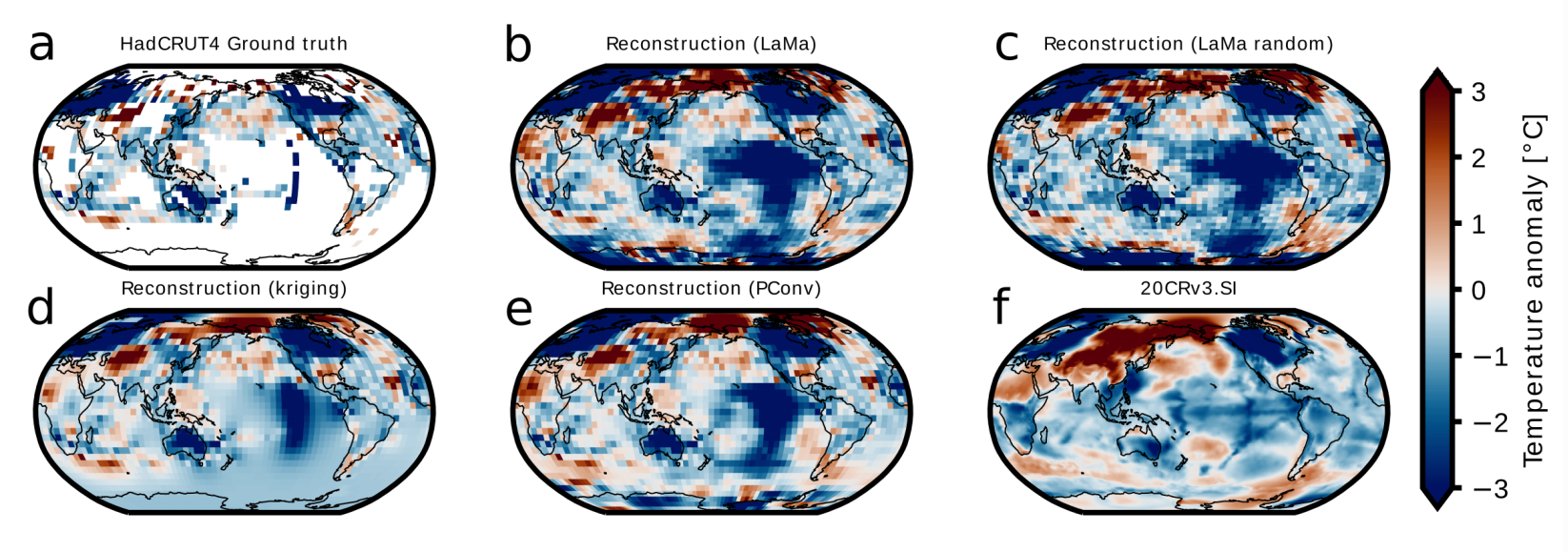
A preprint has appeared on infilling of global temperature data using “deep learning”. On their tests, it performs better than the Kadow et al. method. That’s quite interesting and new methods for filling the gaps in HadCRUT are always great to see. What’s more exciting, potentially, is that they used the same method to infill […]
The International Cryosphere Climate Initiative has put together a new petition for scientists to sign. I’m a little sceptical that this kind of “clicktivism” makes much difference, but there are many many lobbyists from polluting industries at the COP28 and rather fewer scientists. And how else to draw attention to what is one of the most visible and urgent effects of climate change?
The petition is aimed at:
” all cryosphere scientists globally; as well as those working on emissions pathways: and those in the social sciences with research on adaptation, loss and damage and health impacts. This includes research and field associates, as well as doctoral students — because you are the future, and will be dealing with the impacts of climate change in the global cryosphere throughout your lives, as well as your professional careers.”
ICCI
The list of signatories so far already includes many rather senior scientists, so take this as a challenge to add your signature if you work in the cryosphere/climate space. It takes only a minute to sign and there are many familiar names on the list.
I’m not sure how else to emphasise the urgency of real action at COP 28.
As a coincidence though, and as I posted on mastodon the image below appears in Momentum, a plug-in on my web browser with a new photo every day. Today’s is this beautiful image of the Marmolada glacier in Italy by Vicentiu Solomon.
It’s a gorgeous but very sad picture – this is one of the faster disappearing #glaciers in the world and to hear more about the consequences of cryosphere loss, take a look at the policy brief produced by the PROTECT project on the sea level rise contributions from glaciers and ice sheets. It also contains this eye opening graphic:
A 2 metre rise in sea level is almost inevitable. The uncertainty is on the timing which is somewhere between one century and the next 2 thousand years, depending on where you are in the world, but, more importantly given COP28, how fast fossil fuels are phased out. You can download the whole thing here.
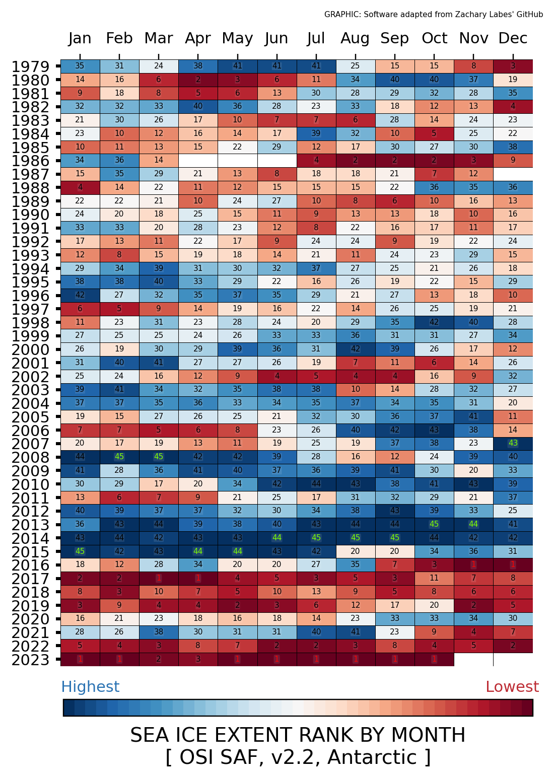
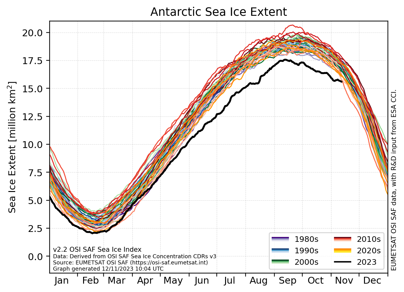
The Danish online popular science magazine is currently running a series on tipping points in the Earth system with a series of interviews with different scientists. They asked me to comment on the extraordinary low sea ice in Antarctica this year. You can read the original on their site here. But I thought it might be interesting for others to read in English the piece which is a pretty fair reflection of my thinking. So I’m experimenting a little with DeepL machine translation which I consider much more reliable that google’s competitor. I have not edited anything in the below! I have been promising a piece on West Antarctica for a while – which I’m still working on, but hopefully this is interestign to read to be going on with!
A sudden and surprising loss of sea ice in Antarctica could be a sign that we are approaching something critical that we need to prepare for, warns an ice researcher from DMI. The climate seems to be changing before our eyes.
In Antarctica, there has been a sudden, violent and in many ways unexplained lack of sea ice, which normally melts in the summer and re-forms in the winter.
Monthly sea ice extent ranked by month also processed by OSI SAF. 2022 and 2023 are both extremely low.
Since then, some of what was lost has been recovered, but when the sea ice peaked in September 2023, 1.75 million square kilometres of sea ice was still missing. This is equivalent to about 40 times the area of Denmark.
“The melting sea ice in Antarctica is not unexpected in itself, because we have long predicted that it would disappear due to global warming,” Ruth Mottram, senior climate researcher and glaciologist at the Danish Meteorological Institute (DMI) tells Videnskab.dk.
The climate seems to be changing before our eyes.
2023 has seen record high temperatures both on land and in the sea, which you can read more about in the article ‘Is the climate running out of control like in ‘The Day After Tomorrow’?
“But to suddenly have a very, very large disappearance like that is a big surprise. We can’t explain why it happened, and our models can’t recreate it either,” she says, but adds that over time, the models are getting closer to reality.
Disturbances in the Earth’s system are probably connected
Videnskab.dk has in a series asked five leading Danish scientists to assess the state of the climate from their chair – in this article Ruth Mottram.
The OCEAN:ICE project The researchers in OCEAN:ICE, led by Ruth Mottram as principal investigator, will take measurements below the ocean surface. This will provide more knowledge about the temperatures in the ocean around Antarctica. They will also calculate how fast the ice is melting in Antarctica due to ocean processes and warming in the air. They will also investigate what the lack of sea ice means for the rest of the Antarctic system. Ruth Mottram cites as examples: How does it affect ecosystems? For example, many animals feed on the small crustacean krill, whose life is affected by sea ice. Will more waves now reach the Antarctic ice sheet and perhaps lead to more icebergs and more melting? Will glaciers and icebergs become more sensitive to heat? Or, on the contrary, will less sea ice trigger more snow over the continent, which could even stabilise the glaciers? More specifically, researchers will focus their efforts on seven areas, which you can read more about on the OCEAN:ICE website.
In the project, researchers will, among other things, take measurements under the sea surface in Antarctica to gain more knowledge about how the ocean and ice interact.
Is melting sea ice linked to warm water in the Atlantic?
In the North Atlantic, sea surface temperatures in some places have been as much as five degrees above normal.
To an outsider, it seems obvious that this could have something to do with melting sea ice.
However, according to Ruth Mottram, the two factors are not necessarily directly related. Sea ice in Antarctica melts from below. Therefore, the temperature at the bottom of the sea is far more important than the temperature at the surface.
“But if there’s one thing I’ve learnt over the past 15 years working at DMI, it’s how interconnected the whole world is. So I think we’re seeing some disturbances throughout the Earth system that are unlikely to be completely independent of each other,” she says to Videnskab.dk.
Ocean Professor Katherine Richardson made the same point earlier in the series. You can read about it in the article ‘Professor: The oceans are warming much faster than expected’.
Lack of knowledge and observations
Ruth Mottram emphasises that far more observations from Antarctica are needed before we can say anything definite about the causes of the rapidly shrinking sea ice, but: “It could indicate that the Antarctic sea ice has a critical tipping point like the Arctic, where for a number of years we see a slow decline year by year, and then suddenly it drops to a new stability where it is very low compared to before.””But we don’t know, because there are parts of the system that we don’t understand and that we haven’t observed yet,” explains Ruth Mottram.
Possible reasons why sea ice is disappearing
Ruth Mottram talks a lot with international colleagues about why the sea ice is currently experiencing a significant decline.
She explains that there are different theories, for example that warmer water from below is coming into contact with the sea ice and melting it from below, and that warmer air may be feeding in from above.
In Antarctica, the direction and strength of the wind has a big impact on the state of the ice (click here for a scientist’s timelapse of how Antarctic weather changes rapidly).
Perhaps the sea ice has been hit by “a very unfortunate event”, where it is both being hit by warm water from below and being affected by weaker winds from changing directions, which is holding back the recovery of sea ice.
Again, more research is needed.
Melting ice also contributes to sea level rise, and the Earth is actually designed so that melting in Antarctica hits the northern hemisphere much harder than melting in Greenland. So, bad news for the ice in Antarctica is bad news for Denmark.
Even more bad news is on the horizon.
The natural weather phenomenon El Niño looks set to get really strong over the next few months. A so-called Super-El Niño will likely only make the world’s oceans even warmer.
“We know that the ocean is going to be really, really important in the future in terms of how fast the Antarctic ice is melting and what that will mean for sea level rise,” says Ruth Mottram. We can’t just wish the world would look different
The climate scientist does not fear huge increases or a violent change in climate overnight, as depicted in the 2004 disaster film ‘The Day After Tomorrow’. She points out that even abrupt shifts in the Earth’s past climate have occurred over decades or centuries, not a few months or years. Still, Ruth Mottram thinks it makes sense to start talking a little more openly about how we tackle severe sea level rise – which on a smaller scale can still be sudden – and large-scale climate change.
The Antarctic ice sheet is the largest on the planet
Figure made on http://www.thetruesize.com showing how Antarctica is roughly 1.5 times the size of the USA.
The Antarctic ice sheet contains around 30 million cubic kilometres of ice. This means that around 90 per cent of all fresh water on Earth is frozen in Antarctica.
If all the ice sheet in Antarctica melts, the world’s oceans will rise by around 60 metres. Even if we stay within the framework of the Paris Agreement, we risk that melting Antarctic ice from Antarctica will cause sea levels to rise by 2.5 metres.
Ruth Mottram notes that the more we exceed the limits of the Paris Agreement, the faster sea levels rise – and slower if we act quickly and stay close to the set limits of preferably 1.5 and maximum 2 degrees of temperature rise compared to the 1800s.
“The Earth’s climate system may be shifting towards a new equilibrium, which could result in a different world than we have grown up with,” continues Ruth Mottram.
“It is already affecting us and will do so increasingly in the future. That doesn’t mean it will be a total disaster, but we will probably get to the point where we have to adjust our lifestyles and societies.”
“It won’t necessarily be simple or easy to do so, but we can’t just wish for the world to be different than it is,” says Ruth Mottram.
“We are in the process of allowing future generations to accept that large areas of land will become uninhabitable because the water level rises too much,” he says. ‘Bipolar’ researcher: Keep an eye on Greenland too
In the short term, Ruth Mottram is interested in finding out what the consequences of El Niño will be and how Antarctica will change over the next few years.
But she also has her sights set on Greenland.
“Because there have been so many weather events elsewhere, it has gone a bit unnoticed that we’ve had a really high melt season in Greenland this year.
“It can give us the opportunity to see very concretely how weather and climate are connected. That’s why the next few years will be really interesting in Greenland,” says Ruth Mottram, who has also conducted research in the Arctic for many years.
The next article in Videnskab.dk’s series on the state of the climate will focus on Greenland.
If you follow me on mastodon you may have noticed a higher than normal number of posts, boosts and the like, many of them dealing with train travel in Europe.
View from a bridge: crossing the Great Belt Bridge (Storebæltsbroen) on the way to Germany
It is annual meeting season and that means the Horizon Europe projects I’m involved in (PolarRES, PROTECT, OCEAN:ICE) are gathering together somewhere more or less central (this year the Netherlands is popular) and discussing, presenting and planning with consortia members is going full speed ahead. After the pandemic when projects started online only or were written entirely via online meetings, even involving people who had never met each other, it’s clearly past time to come together in-person and discuss the newest findings.
I am involved in many different projects in varying roles (work package lead, project scientist, project coordinator). I find these meetings are incredibly stimulating and challenging. They help to get the scientific creativity going, to make new connections and meet new researchers, often early career scientists with new ideas and new techniques. Often this is an opportunity to see results that will not appear in the literature for months or years, as well as being an opportunity for planning new work.
On the way to Utrecht for PolarRES annual meeting. The first train of the meeting season was a Deutsche Bahn IC train loaned by Danish operator DSB to cope with increased demand between Copenhagen and Hamburg.
They’re also exhausting, often starting 8.30am and nominally finishing at 6pm but with many delegates in the same hotels and meeting over breakfast, not to mention late into the evening discussions over dinner, the days are long and non-stop.
I suspect it is much worse for those who do not have English as a first language. My Danish is fairly fluent these days, but I know how tiring it is to speak a foreign language all day. At the end all you want to do is crawl away to a dark room with no sensory stimulation at all..
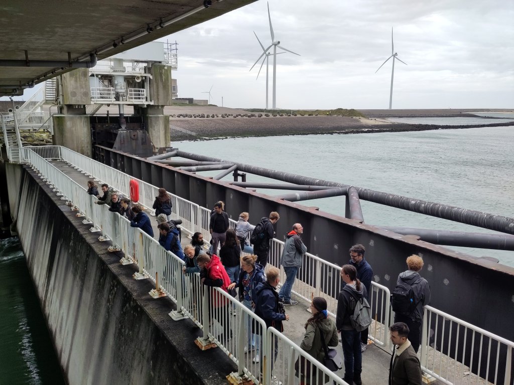
The PROTECT project on sea level rise contributions from the cryosphere had a field trip this year, to the Eastern Scheldt Barrier, a wonder of the modern world and really frontline when it comes to European sea level rise adaptation. Inspiring to see how our work can be applied but also an opportunity for networking and informal discussions
This year, as in other years, I’m trying to do as much travelling as possible by train. It’s actually a nice way to travel to meetings, with plenty of time and space to get work done while travelling.
Far more pleasant than flying, with more legroom, space to move about and without the ridiculous security queues. I use my time to prepare presentations for the meeting and reflect and follow up from them on the way home as well as to (try) to keep my inbox under control..
(I have notably failed at this task this year, but on the up side I’ve drafted or contributed to 3 different papers, which I think/hope will endure a bit longer than my emails.)
An impromptu dinner meeting: also an opportunity to write papers and see how colleagues write their code.
The Deutsche Bahn trains are particularly pleasant, especially the ICE including buffet cars, excellent food and nice spacious train seats with good WiFi. The TGV was by comparison a little disappointing in terms of comfort but a nice smooth ride. Let’s not get into a discussion on punctuality..
Relaxing on the way home in the dining car with Deutsche Bahn’s finest vegan pasta and a good (actually *excellent*) book. Skål.
Train tickets can be surprisingly economical compared to flying, though usually the plane wins on money and time alone. My current trip from Copenhagen cost a mere 18 euros to get to Hamburg and the sleeper train connection to (near) Paris actually saves money as a berth turns out to be far less than the Paris hotel room I otherwise would have stayed in.
It is, however, aggravating how few sleeper connections there are between major European cities. Surely a connection to Brussels at least if not also Amsterdam makes sense? Props to the Austrian railways for keeping the sleepers alive at all in northern Europe.
There is a toll on family life from flying less. Although my family is growing more independent, the series of meetings have not made me popular at home, and probably rightly so. Travelling by train even to somewhere relatively close like the Netherlands or Paris easily adds a day either side. Letting the train take the strain turns out to also lead to strain on partners and children. In this I have to more than acknowledge my husband who is taking on far more than his fair share this month and who is also extremely supportive when it comes to the extra time.
I imagine not all employers are as tolerant of the extra day on either side travelling either, though as I said, it’s often quite productive, without meetings and office interruptions. Certainly, most of the other scientists have travelled by train from London, Vienna, Grenoble and even Kyiv.
A sleeper connection from city centre to centre would make all these links much more bearable from both points of view.
Even the few remaining sleepers leave only from Hamburg, not Copenhagen. That means a 4.5 hour (on a good day, it can be up to 6 hours on a slow train) each way connection to Copenhagen to factor in. Though, I should give an honourable mention to the Snälltaget, whose Stockholm- Copenhagen -Hamburg -Berlin service has been so popular it is now a year round service after being a temporary summer trial.
Don’t get me wrong, I quite like Hamburg, it is, if not charming, certainly culturally vibrant and a melting pot to rival London (let’s not forget it’s where the Beatles learnt their trade) and there is some excellent food and drink at the station. I’m practically at the Syrian mezze kitchen (seriously, check it out next time you’re passing through). However, it is also a gigantic bottleneck on the railway network and I’ve learned the hard way to allow at least an hour connection time and preferably more ..
Then there is the whole hassle of booking tickets and finding connections. Which is not to be underestimated. As a committed train traveller, I’m pretty good at it now, but it takes a lot of practice and as Jon Worth has eloquently pointed out, particularly when transferring internationally, some rail companies take a perverse delight in senseless connection times..
This is why I am a huge supporter of the Trains for Europe #CrossBorderRail initiative. If we want to reduce flying. And let’s be frank. We MUST, there is no way around it if we want to keep carbon out the atmosphere, then making it easy to replace planes with trains and buses (comfy, long distance ones and where possible electrified) is going to be essential.
And harmonising timetables, tickets and booking across Europe could be the kind of boring stuff that turns out to usher in a kind of quiet revolution in transport…
UPDATE THE MORNING AFTER (21/10/2023): water levels are now falling rapidly to normal and the worst of the gales are past, so it’s time for the clean-up and to take stock of what worked and where it went wrong. It’s quite clear that we had a hundred year storm flood event in many regions, though the official body that determines this has not yet announced it. Their judgement is important as it will trigger emergency financial help with the cost of the clean-up.
In most places the dikes, sandbags and barriers mostly worked to keep water out, but in a few places they could not deal with the water and temporary dikes (filled pvc tubes of water km long in some cases) actually burst under the pressure, emergency sluice gates and pumps could also not withstand the pressure in one or two places.
Trains and ferries were delayed or cancelled and a large ship broke free from the quayside at Frederikshavn and is still to be shepherded back into place.
Public broadcaster DR has a good overview of the worst affected places here.
Water levels reached well over 2m in multiple places around the Danish coast and in some places, water measurements actually failed during the storm..
In other places, measurements show clearly that the waters are pretty rapidly declining. So. A foretaste of the future perhaps? We will expect to see more of these “100 year flood” events happening, not because we will have more storms necessarily but because of the background sea level rising. It has already risen 20cm since 1900, 10cm of that was since 1991, the last few years global mean sea level has risen around 4 – 4.5 mm per year. The smart thing to do is to learn from this flood to prepare better for the next one.
But we as a society also to assess how we handle it when a “hundred year” flood happens every other year…
-Fin-
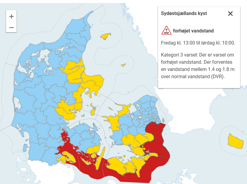
Like much of northern Europe we have been battening down the hatches, almost literally, against storm Babet in Denmark this week. DMI have issued a rare red weather warning for southern Denmark, including the area I often go kayaking in.
Weather warning issued by DMI 20th October 2023 There are three levels, blue signifies the lowest, yellow is medium and the highest is red, which is rather rarely issued. The boxed text applies to the red zome around southern Denmark and states it relates to a water level of between 1.4 and 1.8m above the usual.
I should probably start by saying that this storm is not caused by climate change, though of course in a warming atmosphere, it is likely to have been intensified by it, and the higher the sea level rises on average, the more destructive a storm surge becomes, and the more frequent the return period!
Neither are storm surges unknown in Denmark -there is a whole interesting history to be written there, not least because the great storm of 1872 brought a huge storm surge to eastern Denmark and probably led directly to the founding of my employer, the Danish Meterological Institute. My brilliant DMI colleague Martin Stendel persuasively argues that the current storm surge event is very similar to the 1872 event in fact, suggesting that maybe we have learnt something in the last 150 years…
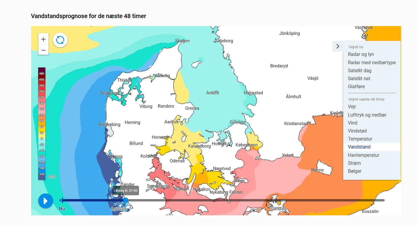
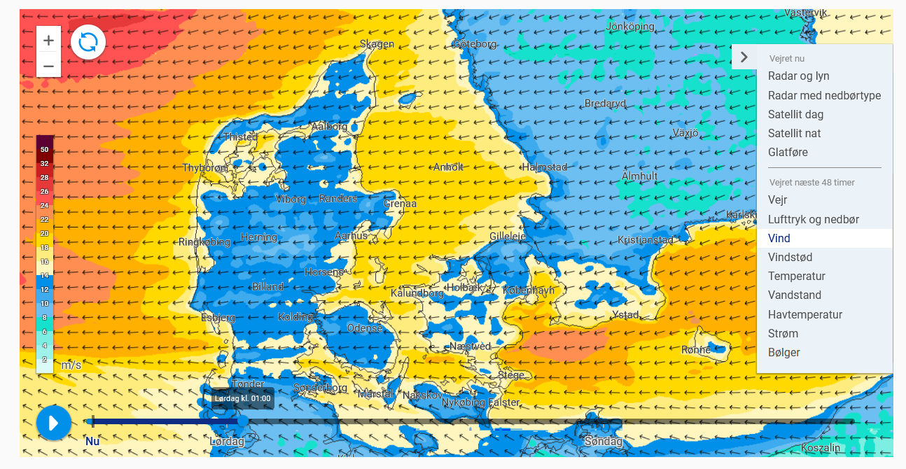
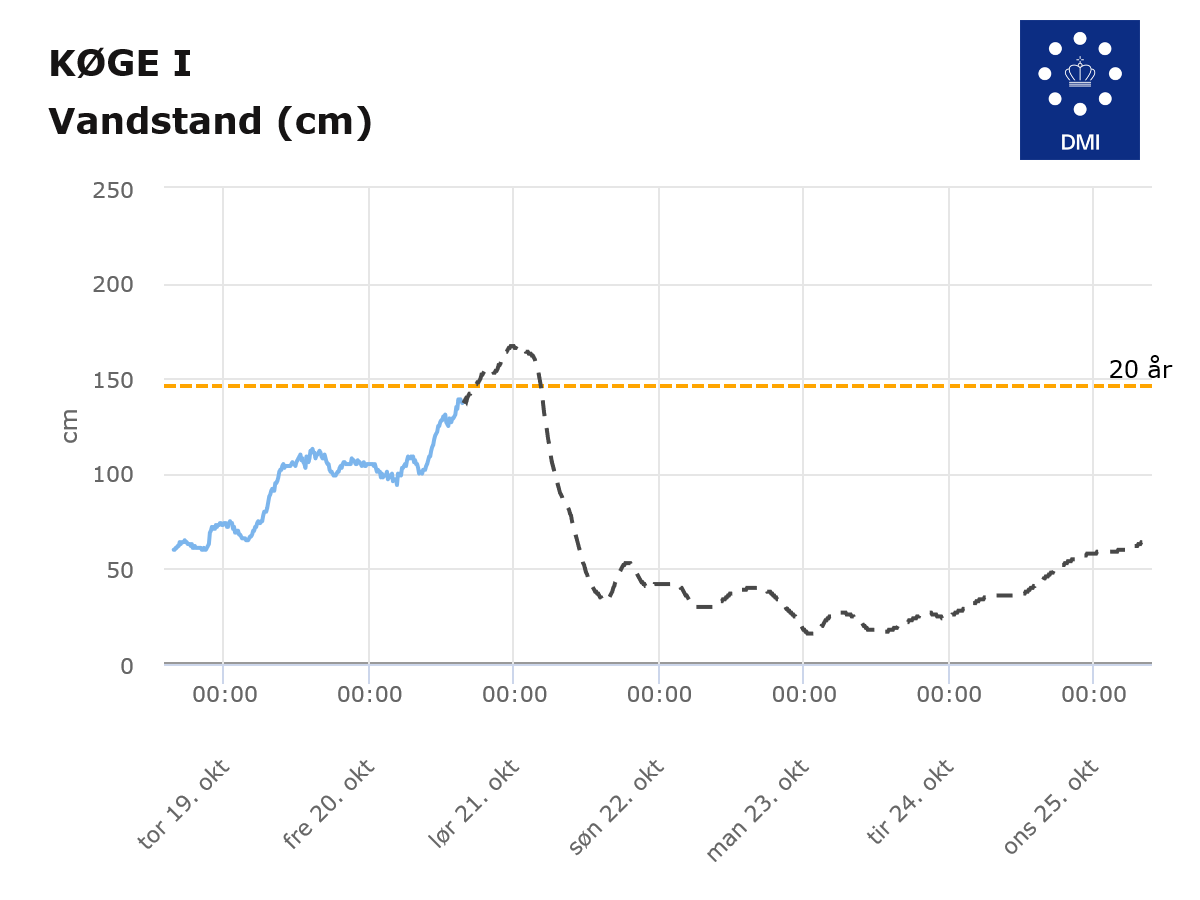
However, back to today: the peak water is expected tonight, and the reason why storm surges affect southern and eastern Denmark differently to western Denmark is pretty clear in the prognosis shown below for water height (top produced by my brilliant colleagues in the storm surge forecasting section naturally) and winds (bottom, produced by my other brilliant colleagues in numerical weather prediction):
Basically, the strong westerly winds associated with the storm pushed a large amount of water from the North Sea through the Kattegat and past the Danish islands into the Baltic Sea over the last few days. Imagine the Baltic is a bath tub, if you push the water one way it will then flow back again when you stop pushing. Which is exactly what it is now doing, but now, it is also pushed by strong winds from the east as shown in the forecast shown above. These water is being driven even higher against the coasts of the southern and eastern danish islands.
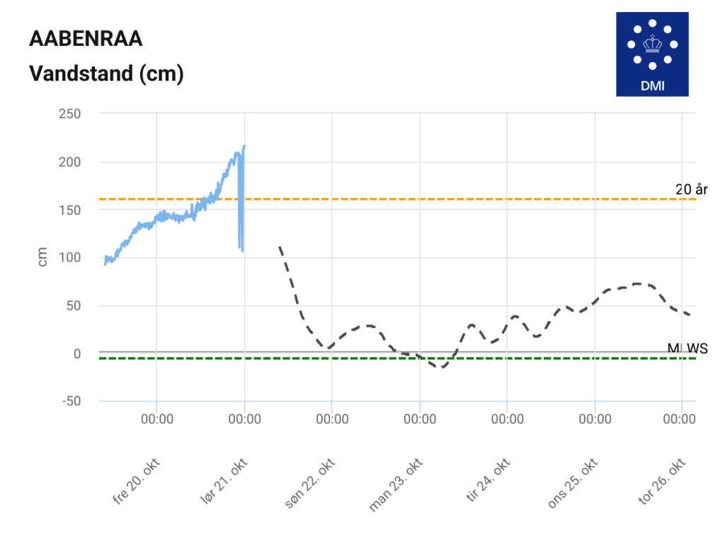
These kind of storm surges are sometimes known as silent storm surges by my colleagues in the forecasting department because they often occur after the full fury of the storm has passed. I wrote about one tangentially in 2017. This time, adding to the chaos, are those gale force easterly winds, forecast to be 20 – 23 m/s, or gale force 9 on the Beaufort Scale if you prefer old money, which will certainly bring big waves that are even more problematic to deal with that a slowly rising sea, AND torrential rain. So while the charts on dmi.dk which allow us to follow the rising seas (see below for a screengrab of a tide gauge in an area I know fairly well from the sea side), water companies, coastal defences and municipalities also need to prepare for large amounts of rain, that rivers and streams will struggle to evacuate.
Water height forecast for Køge a town in Eastern Sjælland not far from Copenhagen. The yellow line indicates the 20 year return period for this height. Blue line shows measurements and dashed black lines show the forecast from the DMI ocean model. You can find more observations here.
In Køge the local utilities company is asking people to avoid running washing machines, dishwashers and to avoid flushing toilets over night where possible to avoid overwhelming sewage works when the storm and the rain is at the maximum.
This brings me to the main lessons that I think we can learn from this weather (perhaps super-charged by climate) event.
Firstly, it’s the value of preparedness, and learning from past events. There will certainly be damage from this event, thanks to previous events, we have a system of dykes and other defence measures in place to minimse that damage and we know where the biggest impacts are likely to be.
Secondly, the miracle, or quiet revolution if you will, of weather and storm forecasting means we can prepare for these events days before they happen, allowing the deployment of temporary barrages, evacuations and the stopping of electricity and other services before they become a problem.
This is even more important for the 3rd lesson, that weather emergencies rarely happen alone – it’s the compound nature of these events that makes them challenging – not just rising seas but also winds and heavy rain. And local conditions matter – water levels in western Denmark are frequently higher, the region is much more tidally influenced than the eastern Danish waters. This is basically another way of saying that risk is about hazard and vulnerability.
Finally, there are the behavioural measures that mean people can mitigate the worst impacts by changing how they behave when disaster strikes. Of course, this stuff doesn’t happen by itself. It requires the slightly dull but worthy services to be in place, for different agencies to communicate with each other and for a bit of financial head room so far-sighted agencies can invest in measures “just in case”. We are fortunate indeed that municipalities have a legal obligation to prepare for climate change and that local utilities are mostly locally owned on a cooporative like basis – rather than having to be profit-making enterprises for large shareholders..
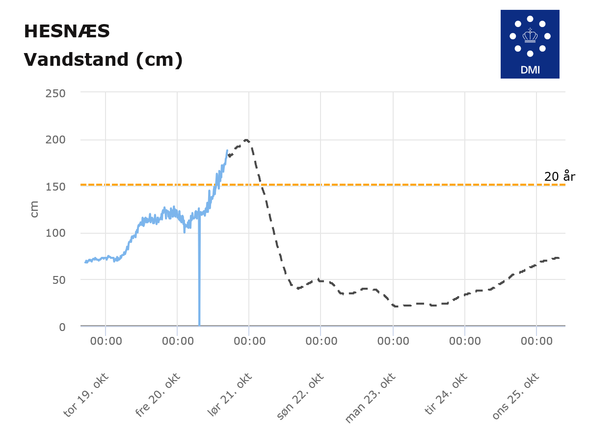
This piece is already too long, but there is one more aspect to consider. The harbour at Hesnæe Havn has just recorded a 100 year event, that is a storm surge like this would be expected to occur once ever hundred years, in this case the water is now 188cm. The previous record of 170cm was set in 2017. We need to prepare for rising seas and the economic costs they will bring. The sea will slowly eat away at Denmark’s coasts, but the frequency of storm surges is going to change – 20cm of sea level rise can turn a 100 year return event into a 20 year return event and a 20 year return event into an ever year event.
Screenshot of the observations of sea level from Hesnæs
We need to start having the conversation NOW about how we’re going to handle that disruption to our coastlines and towns.
Following the invasion of Ukraine, Arctic exceptionalism is no longer. The region is reproducing deep divisions between Russia and the West in lower latitudes.